Geospatial Raster Analysis in R

LearningLearning Objectives

After completing this session, you will be able to:

• Describe the key spatial parameters of a raster (coordinate reference system, extent, resolution, and origin) and explain why they must align across rasters used in a common analysis
• Create raster objects in R from multiple starting points, including GeoTIFF files, tabular x-y data, vector polygons, and manually specified parameters
• Apply raster math and logical indexing to calculate derived metrics such as NDVI directly from raster layers
• Modify raster spatial parameters using crop(), mask(), aggregate(), resample(), and project()
• Extract and summarize raster values using vector spatial data as a selection criterion using extract()
• Convert between raster and data frame formats to enable tidyverse-style analysis workflows and ggplot2 visualization

1 Scope: Raster, Not Vector

This lesson focuses on working with raster spatial data in R, primarily using the terra package in R. Raster data is typically a grid of pixels with each pixel containing some value of a continuous variable, like elevation or temperature. Satellite imagery and remote sensing data are common examples of raster data. This is distinct from vector spatial data, such as points, lines, and polygons, which are not constrained to a grid but have challenges of their own.

In this overview of raster spatial data, we will introduce basic concepts of creating rasters, modifying them, and doing basic analyses with them. While this lesson does not focus on working with vector spatial data, we will use some vector spatial data (using the sf “Simple Features” spatial package) in conjunction with our raster analysis.

Vector spatial data

Raster spatial data

Figure 1: Image Source - National Ecological Observatory Network (NEON)

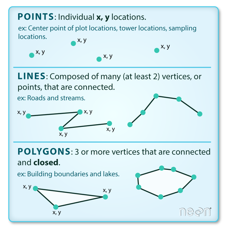
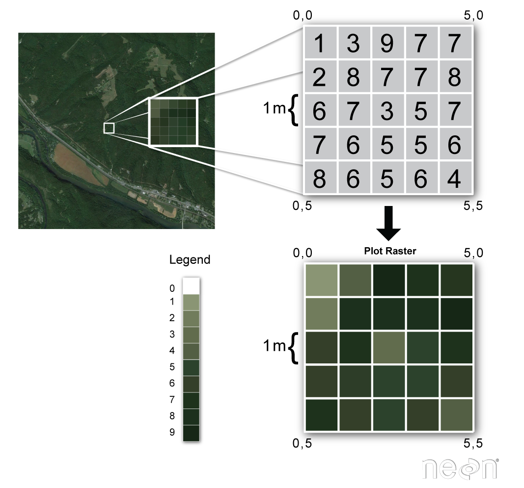
Mastering spatial data in R (or any GIS system) requires a solid understanding of both vector and raster spatial data.

Noteterra vs. raster vs. stars

The terra package is the current standard for working with single- and multi-layer raster data, replacing the older (but still functional) raster package without a lot of friction, and more intuitive as a starting point.

The stars package is a massive overhaul of raster-style data for R to work more seamlessly with data arrays in a manner similar to sf for vector data. Once you’re familiar with terra, stars is an alternative worth exploring for array-oriented or time-series raster data such as time series satellite imagery.

2 Set Up a New Quarto Document

Create a blank Quarto document in your desired repository.

Positron

1. In Positron, go to File New File Quarto Document.
2. Update the YAML header with title, author, and other desired fields. Delete any boilerplate below the YAML.

RStudio

1. In RStudio, go to File New File Quarto Document.
2. Give it a title (e.g., “Introduction to Quarto”), leave the other options as-is, then click Create.
3. Update the YAML header with title, author, and other desired fields. Delete any boilerplate below the YAML header.

For this lesson, we will need to load a few packages. You may want to put code options in the code chunk, e.g., #| message: false and #| warning: FALSE

### for easy data wrangling and plotting:
library(dplyr)     
library(tidyr)
library(ggplot2)
### spatial data packages:
library(terra)     ### for working with raster spatial data
library(sf)        ### for working with vector spatial data
### for easy relative file paths:
library(here)     

3 Let’s Create a Raster!

As with many things in R, there are many ways to create rasters depending on the information you have to start:

• Read in a file in a raster-ready format, e.g., GeoTIFF or NetCDF
• Read in a dataframe with x, y, and value columns and convert to a raster
• Rasterize a vector layer, e.g., lines representing rivers or polygons representing zones
• Create a raster from scratch by providing the necessary parameters
• … and more!

3.1 Raster Spatial Parameters

There are several parameters that every raster must have:

• Coordinate reference system (CRS): A system to locate things spatially on the surface of the earth - basically a definition of the shape of the globe (hint: not a sphere), some way to identify where X = 0 and Y = 0, and quite likely some projection to convert curved space into flat space. Includes units, usually degrees or meters.
• Resolution: The length of the sides of each grid cell, in both X and Y. This is in units given in the coordinate reference system.
• Origin: The offset of the grid from (0, 0) (as given in the CRS), or alternately, the point closest to (0, 0) that you could get to by moving in steps of the x and y resolution.
• Extent: The corners of the rectangular box that bounds your raster.

If you want to use multiple rasters in an analysis, these spatial parameters must match up across every raster, so the software can directly match and compare corresponding cells in different layers.

3.2 Creating a Raster: Four Ways

From Gridded File Format

Download this LandSat sample data - note the file format is .tif, i.e., a GeoTIFF. Right click on the link, choose “Save link as…”, and save it to your data folder in your current repository as landsat71.tif.

Now let’s load it and examine it!

landsat_r <- terra::rast(here('data/landsat71.tif'))

Inspect the Parameters

landsat_from_tif

class       : SpatRaster
size        : 1758, 3701, 5  (nrow, ncol, nlyr)
resolution  : 30, 30  (x, y)
extent      : -59564.57, 51465.43, -404675.9, -351935.9  (xmin, xmax, ymin, ymax)
coord. ref. : NAD83 / California Albers (EPSG:3310)
source      : landsat71.tif
names       : landsat71_1, landsat71_2, landsat71_3, landsat71_4, landsat71_5
min values  :           0,           0,           0,           0,           0
max values  :         255,         255,         255,         255,         255

This SpatRaster object created from a GeoTIFF file contains gridded data for five bands of Landsat data for Santa Barbara County: blue 450 nm - 520 nm (band 1), green (band 2), red (band 3), near-infrared (band 4), and shortwave-infrared (band 5). Examine the parameters.

Plot the Layers

plot(landsat_from_tif)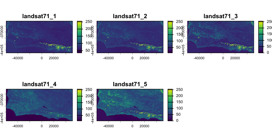

It may be hard to tell the differences in this view, but we can see five distinct maps.

From X-Y Coords

We can create a raster from a dataframe (or other formats using) X-Y coordinates (e.g., lat/long or meters E/meters N) - as long as they’re on a regular grid.

Download this .csv of modified LandSat sample data - note the file format is .csv - and save it to your data folder in your current repository as landsat71_band2.csv.

Now let’s load it and examine it!

ls_green_df <- readr::read_csv(here('data/landsat71_band2.csv'))

Examine the dataframe: columns for x, y, and Landsat band 2, green. We can easily turn this into a raster using terra::rast(), the same function as above, which recognizes the appropriate columns (though x and y MUST be first by default!).

ls_green_from_csv <- terra::rast(ls_green_df)

Inspect the Parameters

ls_green_from_csv

class       : SpatRaster
size        : 87, 185, 1  (nrow, ncol, nlyr)
resolution  : 600, 600  (x, y)
extent      : -59564.57, 51435.43, -404135.9, -351935.9  (xmin, xmax, ymin, ymax)
coord. ref. : 
source(s)   : memory
name        : landsat71_2
min value   :       39.33
max value   :      253.01

This contains similar information as the GeoTIFF we loaded earlier, except note the parameters are slightly different:

• There is only a single layer
• The resolution here is 600m instead of 30m (we did this for file size - GeoTIFF is far more memory efficient! see aggregate() below)
• The CRS is blank! The GeoTIFF includes CRS information embedded in the file, but the CSV does not.

Let’s update the CRS using the EPSG code based on the GeoTIFF version:

crs(ls_green_from_csv) <- 'epsg:3310' 
### could also do crs(ls_green_from_csv) <- crs(landsat_from_tif)

# ls_green_from_csv ### inspect again if you like!

Plot the Layers

plot(ls_green_from_csv)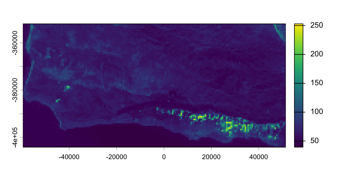

Visually, the pixels are a bit larger; otherwise it looks more or less like the version loaded from the GeoTIFF.

From Vector Data

Download this GeoPackage of Santa Barbara County - note the file format is .gpkg, i.e., vector data like .shp - and save it to your data folder in your current repository as sb_county.gpkg.

Now let’s load it and examine it! We will use the Simple Features package sf.

sb_county_sf <- sf::read_sf(here('data/sb_county.gpkg'))

Examine the resulting Simple Features object: one observation with some random info about Santa Barbara County, and a geometry column containing MultiPolygon spatial information. We can create a raster by overlaying this polygon onto a grid, and then assigning values to the grid based on some attribute.

terra::same.crs(sb_county_sf, landsat_from_tif)  ### Check that CRS are equal!

sb_county_r <- terra::rasterize(x = sb_county_sf,
                                y = landsat_from_tif,
                                field = 'OBJECTID')

1

The vector data to be converted to a raster

2

The target grid, as a SpatRaster object

3

What value gets assigned? Here we assign the value of the OBJECTID field in sb_county_sf, but could be any attribute, or even just a number or vector of numbers.

[1] TRUE

ImportantRaster parameters drive the result!

Note that the north half of SB County is not included in our resulting raster! Because our Landsat raster was used to specify the parameters (including extent), the result gets cropped and some information gets lost. Make sure your vector and raster data play well together!

Inspect the Parameters

sb_county_r

class       : SpatRaster
size        : 1758, 3701, 1  (nrow, ncol, nlyr)
resolution  : 30, 30  (x, y)
extent      : -59564.57, 51465.43, -404675.9, -351935.9  (xmin, xmax, ymin, ymax)
coord. ref. : NAD83 / California Albers (EPSG:3310)
source(s)   : memory
name        : OBJECTID
min value   :        1
max value   :        1

The resulting raster has the same parameters as the y object used to create it!

Plot the Layers

plot(sb_county_r)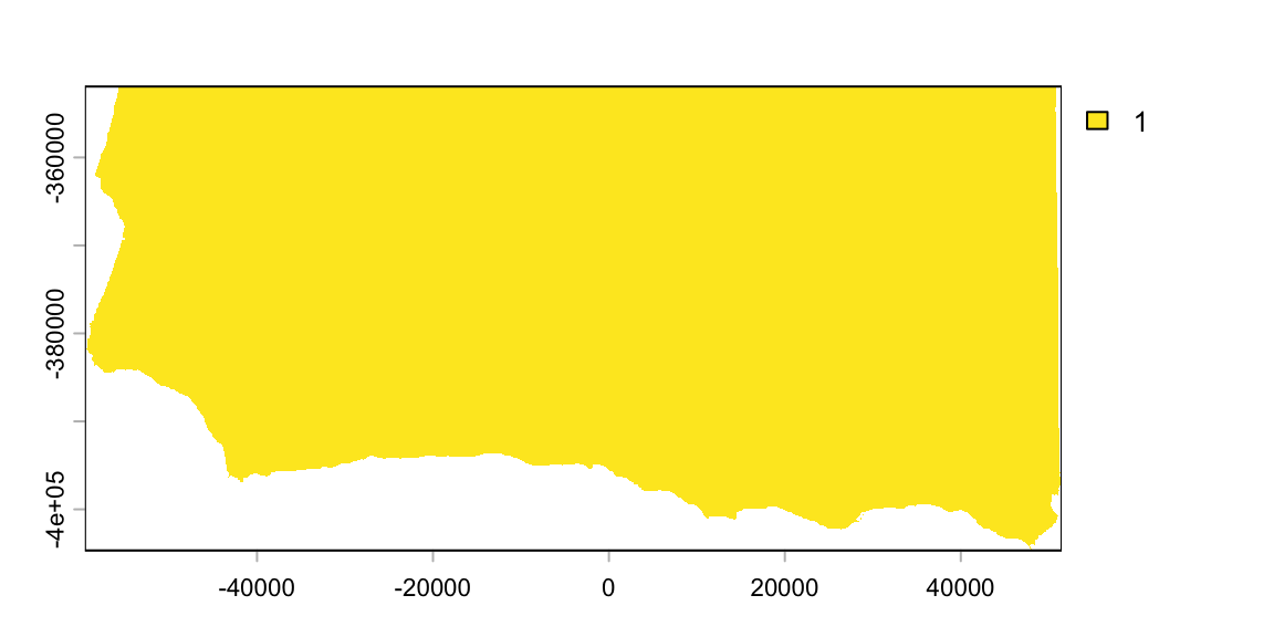

From Scratch

We can also create a raster from scratch, again using terra::rast(). This is useful for creating a blank raster that can be used as a template for rasterizing polygons or lines.

Here, let’s create a global raster, in half-degree pixels, with a unique ID value for each cell, starting with 1 in the upper left. Note we define the parameters manually.

### create the blank template
cellid_r <- rast(xmin = -180, xmax = 180, ymin = -90, ymax = 90,
                 resolution = 0.5,
                 crs = 'EPSG:4326') %>%
  setNames('cell_id')

### set values directly
values(cellid_r) <- 1:ncell(cellid_r)

plot(cellid_r)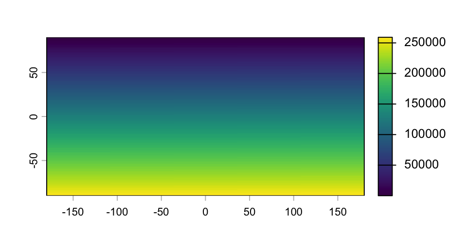

Note, there are many variations on this, e.g., using existing rasters to set the extents and resolution.

NoteSingle-layer vs Multi-layer Rasters

A SpatRaster can hold one or more layers, all sharing the same spatial parameters. Multi-layer rasters are useful for multi-band imagery (like Landsat), time series, or stacking thematic layers. Access individual layers with $name, ['name'], or [[index]].

4 Let’s Do Raster Math!

Rasters are just a grid of numeric values, essentially a matrix, so we can do the same operations on a raster as we can with a basic vector or matrix. Here we’ll walk through some simple examples with a vector then apply the same to our LandSat data.

4.1 Basic Raster Math

### operating on a vector
vec <- 1:10
vec * 2  ### multiply by a scalar

 [1]  2  4  6  8 10 12 14 16 18 20

vec + 20 ### add a scalar

 [1] 21 22 23 24 25 26 27 28 29 30

log(vec) ### transform with a function

 [1] 0.0000000 0.6931472 1.0986123 1.3862944 1.6094379 1.7917595 1.9459101
 [8] 2.0794415 2.1972246 2.3025851

### subset raster using $ or [] notation:
ls_red <- landsat_from_tif$landsat71_3    ### band 3 is red
ls_nir <- landsat_from_tif['landsat71_4'] ### band 4 is near IR

plot(ls_red + 100) ### note color ramp number changed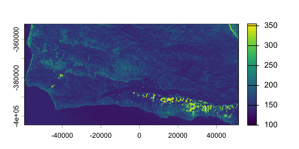

plot(log(ls_red))  ### looks way different!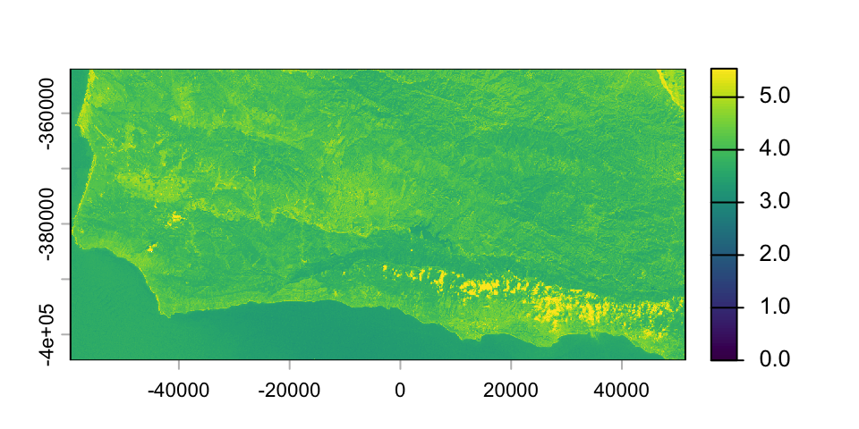

We can also add, subtract, multiply, or divide by a raster with the same spatial parameters, just as we can with vectors.

vec2 <- 100:109
vec / vec2

 [1] 0.01000000 0.01980198 0.02941176 0.03883495 0.04807692 0.05714286
 [7] 0.06603774 0.07476636 0.08333333 0.09174312

plot(ls_red * ls_nir)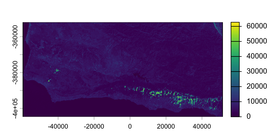

4.2 Raster Indexing

You can also use simple [ ] indexing to change values in raster pixels based on some logical test, or to replace values. Most often, we would find values that DO NOT match our criteria and set them to NA. Here are two examples:

Where is NIR Below 30?

Find cells above 30 and set to NA:

nir_low <- ls_nir ### make a copy
nir_low[nir_low > 30] <- NA ### any NIR value > 30, set to NA
plot(nir_low)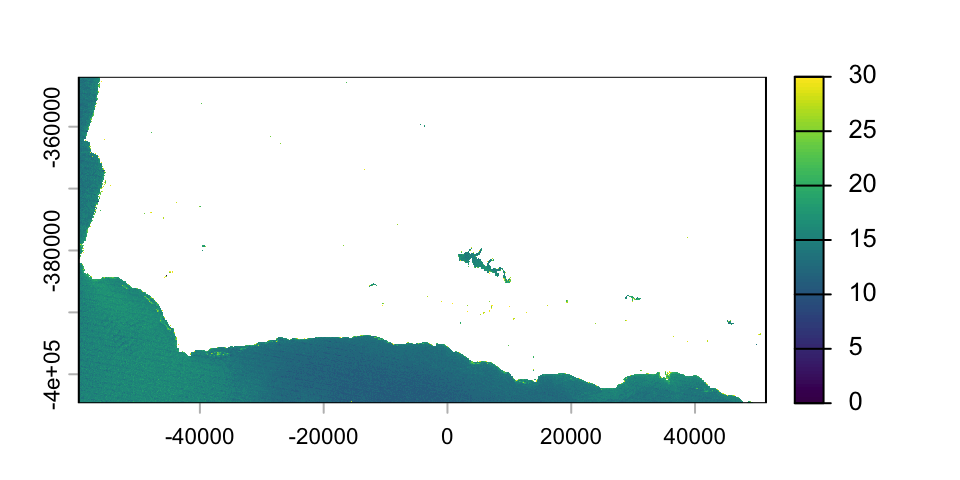

Where is Red Higher than NIR?

Find cells where Red is not higher than NIR and set to NA:

red_hi <- ls_red ### make a copy
red_hi[red_hi < ls_nir] <- NA ### if red < NIR, set to NA
plot(red_hi)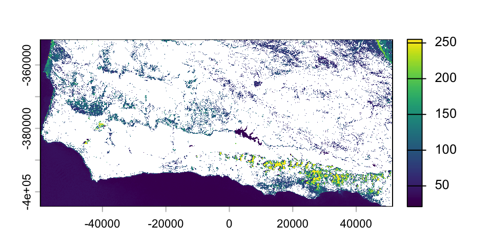

ExampleExample

4.3 Normalized Differential Vegetation Index

Using basic raster math, we can use our red and NIR rasters to calculate the Normalized Difference Vegetation Index (NDVI), a common metric for vegetation health. It works because healthy vegetation strongly reflects near IR while strongly absorbing red, unlike most non-plant matter. The formula is:

\[NDVI = \frac{NIR - Red}{NIR + Red}\]

NDVI Value	Vegetation and Surface Type
-1.0 to 0.1	Water, snow, clouds, or barren rock and sand
0.1 to 0.2	Bare soil or plowed agricultural fields
0.2 to 0.5	Sparse veg, shrubs, grasslands, or senescing crops
0.6 to 0.9	Dense vegetation, healthy crops, or rainforests

Let’s calculate NDVI, then identify vegetated areas using NDVI \(\geq\) 0.2.

NDVI Calculation

Note, here we run the NDVI calculation, then multiply the result using the SB County raster, which drops ocean cells, i.e., where sb_county_r is NA! Note also, we can set a new more informative name for the result using names().

ndvi_all <- (ls_nir - ls_red) / (ls_nir + ls_red) ### all cells
ndvi <- ndvi_all * sb_county_r

names(ndvi) <- 'ndvi'

plot(ndvi)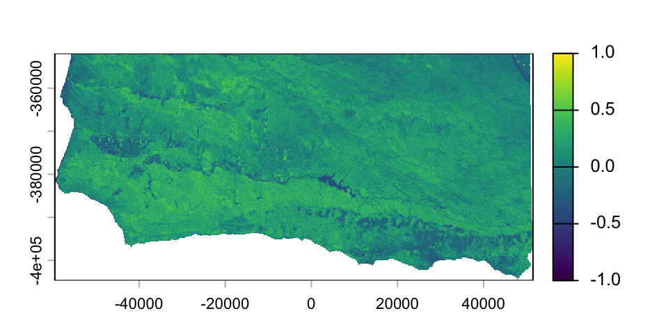

NDVI Filtered and Masked

veg <- ndvi ### create a copy of the NDVI raster so we don't overwrite that!
veg[veg < 0.2] <- NA

plot(veg)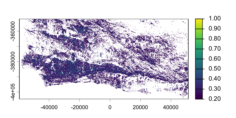

4.4 Summarization Functions

The terra package allows for using basic statistical summary functions directly on rasters at the pixel level.

Max Pixel Value

max_by_pixel <- max(landsat_from_tif)  ### max pixel value across multiple bands
plot(max_by_pixel)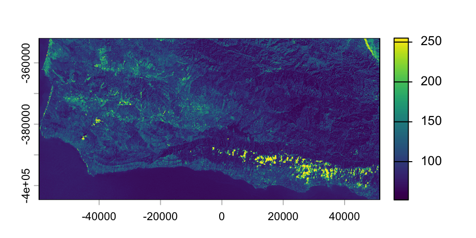

Sum of Pixel Values

sum_by_pixel <- sum(landsat_from_tif)  ### add up values across multiple bands
plot(sum_by_pixel)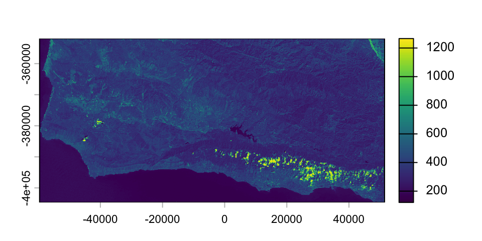

Mean Overall

To get summarized value across the entire map, use values() then apply the summary function:

mean(values(landsat_from_tif))

[1] 69.10275

4.5 Example Use Cases for Basic Raster Math?

• Basic combinations of rasters to quickly calculate ratios, sums, etc.
• Rescale a raster by dividing by the max value: rast_rescale <- rast / max(values(rast))
• Use a raster of presence/absence (as ones and zeros) to turn on or turn off values in a different raster (similar to mask()): rast_masked <- value_rast * presence_absence_rast
• “Flatten” a raster to all ones and NAs by dividing the raster by itself (something divided by itself = 1, 0 divided by 0 = NaN)

5 Modifying Raster Parameters

Raster analysis typically requires all data sources to have identical spatial parameters, but frequently we work with datasets from different sources, using spatial data with different extents, resolutions, and projections.

project()

This is one of the most useful functions for raster analysis. The project() function allows us to reproject the data from one raster into a different extent, resolution, and CRS, using either a target raster or a target CRS. A common use case is when using multiple raster datasets from different sources: define one of your rasters as your “analysis grid” and use project() to convert any other rasters to match extent, resolution, and CRS of your analysis grid.

Because we are translating values from one grid to another, we must specify a method to determine how to resolve differences when cells do not align perfectly:

• near - Nearest neighbor works well for categorical variables, as the spatially closest value is transferred exactly. modal works well too, if multiple input cells overlap with a single output cell.
• bilinear, mean, cubic, and other interpolation methods work well for continuous data.

As an example, let’s reproject our SB county NDVI map, currently in a California Albers projection (in meters, EPSG code 3310), into something obviously wrong: a CRS optimized for Massachusetts spatial data (Massachusetts Mainland Lambert Conformal Conic, in meters, EPSG code 26986). Let’s also change the resolution from 30 m to 2000 m.

ndvi_26986 <- project(x = ndvi, y = 'epsg:26986', res = 2000, method = 'bilinear')
plot(ndvi_26986); plot(ndvi)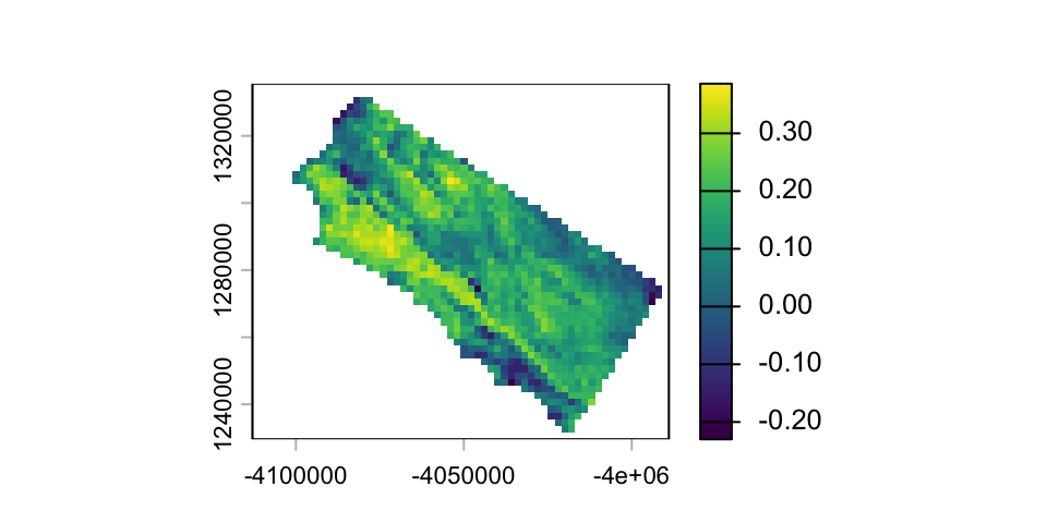

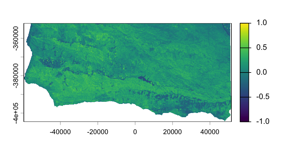
Because we are far from Massachusetts, the distortions caused by the new CRS are plain. We can also see the NDVI values, originally ranging from -1 to 1, are now compressed to -0.20 to +0.40, as extreme values get averaged out due to the bilinear interpolation.

crop()

Sometimes we want to use only a portion of the map. We can crop a raster based on the extents of a different spatial object (SpatRaster, SpatVector, sf, or extent) with the same CRS (but other parameters can be different). Let’s zoom in on the NDVI around Santa Barbara city, rather than the entire county.

Download this GeoPackage of Santa Barbara cities and save it to your data folder in your current repository as sb_cities.gpkg.

sb_city_sf <- sf::read_sf(here('data/sb_cities.gpkg')) %>%
  filter(CITY == 'Santa Barbara')

The rectangular extent or bounding box of the vector data will automatically be applied to crop the raster. Here we plot the raster and then the city boundary on top, to show that values outside the polygon (but within its bounding box) are still included.

ndvi_city <- crop(ndvi, sb_city_sf)
plot(ndvi_city); plot(sb_city_sf %>% select(CITY), border = 'yellow', col = NA, add = TRUE)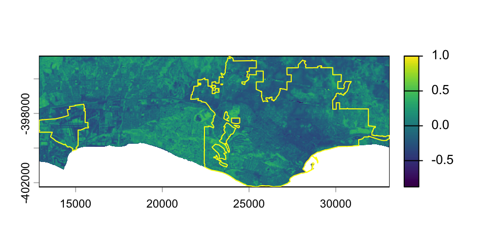

Compare this to mask() below!

resample()

The resample() function is similar to project() in that it transfers values from one SpatRaster grid to another one with different geometric parameters - the difference is that it DOES NOT change the CRS. As for project(), a method must be specified to determine how potential multiple cell values are summarized for the destination cell:

• near - Nearest neighbor works well for categorical variables, as the spatially closest value is transferred exactly. modal works well too, if multiple input cells overlap with a single output cell.
• bilinear, mean, cubic, and other interpolation methods work well for continuous data.

aggregate()

Data at very fine resolution can be computationally challenging to work with - so sometimes it is desirable to make the data more coarse, for example, to more closely match the resolution of another dataset before resampling or reprojecting. The aggregate function is a fast method for converting fine resolution data to coarser resolutions by an integer multiplicative factor, without changing any other parameter.

Our 30 m resolution Landsat data is great, but for a global analysis, something closer to 1 km resolution may be adequate and far more computationally accessible. In a 1 km pixel, you could fit 33.3333 pixels at 30 m (in both x and y). Aggregating by a factor of 33 (integer) gets us to 990 m resolution pixels, using a method to summarize the values of all 30 m pixels within each target 990x990 cell. However, there is a tradeoff, as information is certainly lost in this process.

ls_red_1km <- aggregate(ls_red, fact = 33, fun = 'mean')
res(ls_red_1km)

[1] 990 990

plot(ls_red_1km)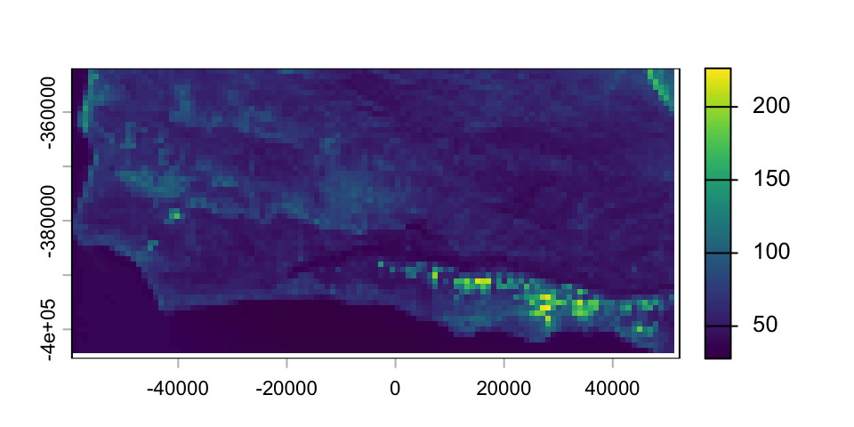

6 Extracting Raster Values

6.1 mask()

Sometimes we want to use one layer (raster or vector) to determine which parts of a raster layer we want to keep, like a stencil: by default, pixels inside the mask layer are kept, while pixels outside are set to NA (though this can be inverted if desired!). Here we use the Santa Barbara city boundary as a mask, to keep only pixels within that boundary. The city boundary is added in yellow, the county boundary is added in red. Note that the extent of the result is unchanged, but all pixels outside the SB city boundary are now blank.

ndvi_city_mask <- mask(ndvi, sb_city_sf)
plot(ndvi_city_mask)
plot(sb_county_sf %>% select(OBJECTID), border = 'red', col = NA, add = TRUE)
plot(sb_city_sf %>% select(CITY), border = 'yellow', col = NA, add = TRUE)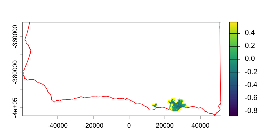

Notecrop() vs mask() vs trim()

• The crop() function changes the extents of a raster based on a target, and retains all data within the new extents.
• The mask() function only retains data that overlap with pixels in the mask layer, but DOES NOT change the extents.
• The trim() function takes an input raster and removes all the outer rows and columns that contain only whitespace - like a crop-to-self. Note, this changes the extent in the process, which may make the result incompatible with other raster layers aligned with the original data.

Try using trim() on the result of our mask() - what happens?

6.2 extract()

To find values of our analysis raster based on some other spatial criteria (e.g., vector polygons/lines/points, xy coordinate), we can use extract(). We can extract values of all cells that meet the criteria, or use the fun argument to apply a statistical function such as mean, min, max, sum to summarize by geometry ID.

NOTE: extract() returns the data as a dataframe instead of a raster, assuming that we are no longer interested in the spatial aspects of our data. But it includes (by default) an ID column that relates to the row numbers of our boundaries (i.e., city boundaries) we are using to extract.

Here we will examine the NDVI values within the boundaries of all cities in Santa Barbara County. We already downloaded this file, and earlier filtered to just Santa Barbara city; let’s load to a new object that includes all cities. Let’s also create a new column called ID that we can use later to bind our city info to our extracted values.

sb_all_cities_sf <- sf::read_sf(here('data/sb_cities.gpkg')) %>%
  mutate(ID = 1:n())

Extract all cell values

Let’s extract the values of all cells within the boundaries of the cities in Santa Barbara County. To extract all values, we leave fun = NULL (default). Then, bind the city info (but drop the geometry column).

ndvi_sb_cities <- extract(ndvi, sb_all_cities_sf, na.rm = TRUE) %>%
  left_join(sb_all_cities_sf, by = 'ID') %>%
  st_drop_geometry()

• What is the maximum NDVI across all cells in the cities of SB? What is the minimum?
• Note, the pixel values have no x or y value - the spatial information has been dropped!

Summarize cell values

Let’s find the mean NDVI values within the boundaries of the main cities of Santa Barbara County. Here we set fun = mean to summarize, rather than leaving it NULL. Then, bind the city info (but drop the geometry column).

ndvi_sb_cities <- extract(ndvi, sb_all_cities_sf, fun = mean, na.rm = TRUE) %>%
  left_join(sb_all_cities_sf, by = 'ID') %>%
  st_drop_geometry()

ndvi_sb_cities %>% select(CITY, ndvi)

           CITY        ndvi
1       Solvang  0.05696764
2      Buellton -0.05036708
3        Lompoc -0.02311393
4        Goleta -0.03519383
5   Carpinteria -0.10408454
6     Guadalupe         NaN
7   Santa Maria         NaN
8 Santa Barbara -0.06177979

• Why are most of these numbers so low? While city greenery would be > 0.2, all the pavement and buildings would have NDVI values below zero, dropping our averages.
• Why are Santa Maria and Guadalupe (in north SB County) both NaN? Because our cities vector spatial data extend beyond the edges of our NDVI data, which focuses on south SB County.

Tip

If we want to find values of our analysis raster based on a different (spatially compatible) raster with the selection criteria, (e.g., a raster of development zone ID, county ID, or country ID), extract() won’t work - we would use the zonal() function instead! In some cases, it may be more efficient to rasterize your spatial criteria and then use zonal() instead of extract().

7 Working With Rasters Data Frames

For more complex analyses, it may be useful to convert rasters into data frames, perform the analysis there, and then convert the results back into a raster. We saw previously how to create a raster from a .csv. This allows the reverse!

7.1 Raster as Data Frame for Calculation

Let’s perform a similar analysis to the NDVI above, this time using the Normalized Difference Water Index (NDWI, McFeeters 1996) to detect water bodies:

\[NDWI = \frac{Green - NIR}{Green + NIR}\]

By this index, values above about 0.3 indicate water bodies, and under indicate non-water areas.

To combine multiple rasters into a single multi-layer raster, simply use the c() function to combine. For this example:

• Combine the green (band 2) and near-infrared (band 4) layers from our Landsat multi-layer raster into a single object. We can access layers in the multilayer landsat using [] or $ indexing using layer names, as above, or [[]] to index using layer number.
  
• Use as.data.frame(xy = TRUE) to convert the raster(s) to a dataframe, creating an X and Y column to hold that information (though the CRS information is lost).
• Use standard data frame wrangling techniques to perform the calculation.
• Then convert back to a raster, reattaching CRS from our original data.

gr_nir_r <- c(landsat_from_tif[[2]], landsat_from_tif[[4]]) %>%
  ### use setNames to rename the two layers!
  setNames(c('green', 'nir'))

gr_nir_df <- as.data.frame(gr_nir_r, xy = TRUE)

ndwi_df <- gr_nir_df %>%
  mutate(ndwi = (green - nir) / (green + nir))

ndwi_r <- rast(ndwi_df, crs = crs(gr_nir_r))

plot(ndwi_r)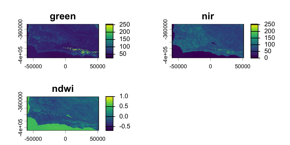

Note that, because our dataframe contained multiple data columns (green, nir, and ndwi, along with x and y), rast() creates a multi-layer raster.

water <- ndwi_r[[3]]       ### create a copy of just the ndwi layer
water[water < 0.3] <- NA ### drop pixels with non-water values
names(water) <- 'water'
plot(water)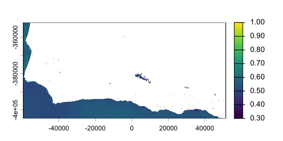

7.2 Raster as Data Frame for ggplot2

Up to now, we have been relying on base::plot() to visualize our rasters. The ggplot2 data visualization package requires inputs to generally be in data frame format. So converting a raster to a dataframe opens this up as a possibility!

ggplot(as.data.frame(water, xy = TRUE)) +
  geom_raster(aes(x = x, y = y, fill = water)) +
  theme_classic() +
  labs(title = 'NDWI for Water Bodies of South Santa Barbara County')

Warning: Raster pixels are placed at uneven horizontal intervals and will be shifted
ℹ Consider using `geom_tile()` instead.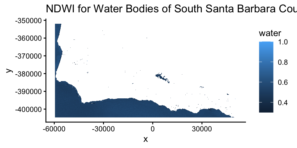

8 Saving Rasters with writeRaster()

Finally, we can write out results of interest using writeRaster(). This looks at the file extension to determine the output format; .tif for GeoTiff is an easy to use format with built-in compression for efficient file sizes.

writeRaster(ndvi, here('data/landsat_ndvi.tif'))
writeRaster(water, here('data/landsat_water.tif'))

9 Summary and Review

• Creating Rasters
  • terra::rast() to load a raster from a file with appropriate format
  • terra::rast() to create a raster from a dataframe with x, y, and value columns
  • crs() <- (or set.crs()) to assign a CRS to a raster using an EPSG code
  • terra::rasterize() to rasterize a vector polygon to a raster grid
  • terra::rast() to create a raster from scratch by specifying extent, resolution, and CRS, and populate it with values using values() <- (or set.values())
• Raster Math and Indexing
  • Math functions (e.g., *, +, log()) to directly modify raster values
  • $, [], and [[]] indexing to extract individual layers from a multi-layer raster
  • Logical indexing (raster[raster > x] <- NA) to mask out values by threshold
  • Multi-layer summary functions (max(), sum()) to summarize across layers pixel-by-pixel
• Modifying Raster Parameters
  • terra::project() to reproject a raster to a new CRS and resolution
  • terra::crop() to crop a raster to the bounding box of a vector or raster
  • terra::aggregate() to aggregate a fine-resolution raster to a coarser resolution
• Selecting Data from Rasters
  • terra::mask() to retain only cells overlapping a vector boundary or raster
  • terra::extract() to extract (and optionally summarize) raster values within vector polygon boundaries
• Rasters and Data Frames
  • as.data.frame(xy = TRUE) to convert a raster to a data frame for use in dplyr workflows
  • ggplot2::geom_raster() to visualize a raster after converting it to a data frame
• Saving Outputs
  • terra::writeRaster() to save out a raster to a file