Machine Learning with tidymodels – 2026 Delta Synthesis Working Groups week 3 (April 2026)

Learning Objectives

After completing this session, you will be able to:

Explain the purpose of partitioning data into training, validation/assessment, and test sets, and describe why this practice helps prevent overfitting
Apply rsample::initial_split() and rsample::vfold_cv() to partition and resample a dataset
Construct classification models using parsnip, applying a consistent syntax across multiple algorithms
Evaluate model performance using appropriate classification metrics
Compare multiple model specifications and algorithms using cross-validated performance metrics to select a best-performing model.
Distinguish between model parameters and hyperparameters, and describe at a conceptual level how tuning strategies search hyperparameter space

1 Overview

Machine Learning (ML) is an intersection between statistics and computer science in which we train computers to learn directly from data without relying on hard-coded rules - identifying patterns, using those patterns to make predictions, then testing those predictions to refine future predictions. ML enables scientists to process, integrate, and analyze datasets across biological, environmental, and socioeconomic domains, helping identify ecological patterns and trends to inform conservation decisions.

Machine learning can range from “stats 101” concepts like linear regression and principal component analysis, to cutting-edge neural networks and transformer models that underpin social media recommendations, large language models, and generative AI.

In this lesson we will explore machine learning in R by applying the tidymodels framework to some relatively simple, intuitive datasets and algorithms.

Scope: Machine Learning Process, not Algorithms

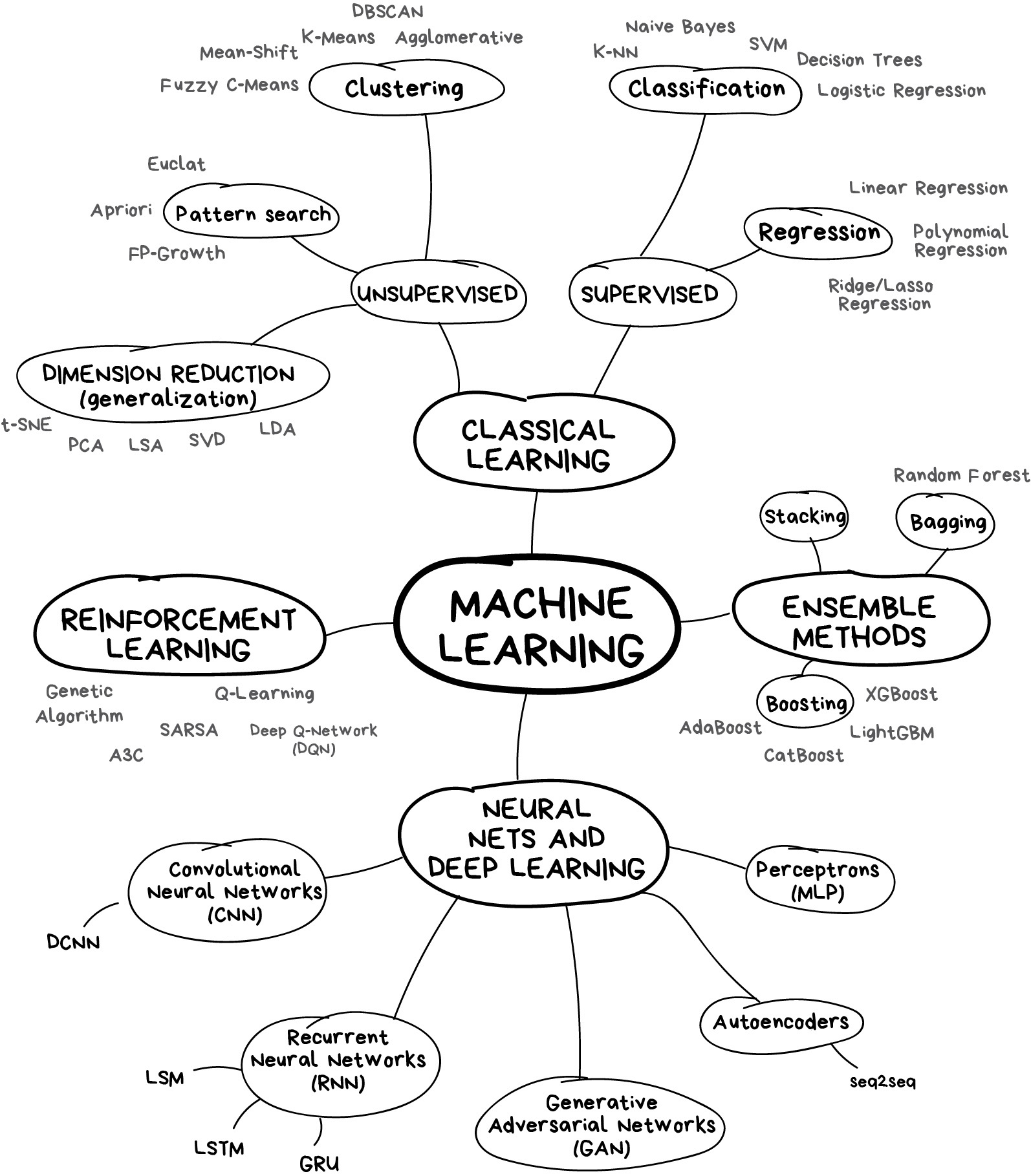
There are far too many possible machine learning algorithms spread across too many R packages to discuss in depth here. Instead, we will focus on a general framework for machine learning that is broadly applicable across model types and algorithms.

2 Machine Learning Overview

Full Screen

An Entertaining Reference

https://vas3k.com/blog/machine_learning/ - This entertaining and informative high-level overview of machine learning, in a similar vein to XKCD or Wait but Why, provides conceptual descriptions of how various ML algorithms work and concrete real-world examples of how you might encounter them in the wild.

3 Setup

3.1 Intro to `tidymodels` and Component Packages

Dozens, maybe hundreds of R packages exist that implement various machine learning techniques, but most of these packages rely on idiosyncratic data input requirements, custom model formats, and different default parameters, making it difficult to use models interchangeably. The tidymodels metapackage and framework do the hard work of consolidating the most popular and frequently used machine learning packages with consistent syntax, inputs, and outputs.

Like the tidyverse, the tidymodels package is actually a collection of many sub-packages each with its own area of expertise. Some of the core packages:

rsample: Handles data splitting and resampling - divide data into training and testing sets, select cross-validation folds, and perform bootstrap sampling for validating model performance
parsnip: Provides a unified, consistent interface for model training - use parsnip functions to specify the model type (e.g., “random forest”) and computational engine (e.g., choose random forest implementation in ranger vs randomForest packages), while maintaining consistent input formats and output formats
workflows: Bundles your data preprocessing steps (recipes) and your model specifications (parsnip) into a single, cohesive object - streamlining the process of fitting and predicting across multiple model algorithms and specifications
yardstick: Evaluates model performance - metrics like accuracy, RMSE (Root Mean Square Error), and ROC AUC to test the predictive power of ML models

3.2 Data Overview

Many machine learning algorithms feel pretty much like a “black box”: data secret magic wisdom. To help develop an intuition of the machine learning process (if not quite the algorithms), we will use a simple and familiar dataset, the palmerpenguins dataset. We will focus on a classification task: identifying the sex of a penguin (harder than it sounds!) from readily observed biometric characteristics.

3.3 Attach Packages and Load Data

library(dplyr)
library(tidymodels) 

### install packages for ML algorithm engines
# install.packages('ranger')
# install.packages('kernlab')

### Load package for penguins data
library(palmerpenguins)

penguins_clean <- penguins %>%
  drop_na() %>%
  ### convert characters to factors - generally easier for modeling engines!
  mutate(species = factor(species), sex = factor(sex), island = factor(island))

# table(penguins_clean$sex)
# # female   male 
# #    165    168 
# table(penguins_clean$species)
# # Adelie Chinstrap    Gentoo 
# #    146        68       119

4 Data Partitioning

One fundamental task of machine learning is dividing data into several discrete, non-overlapping bundles, so we can train our algorithms on one set and then test it against another set. These slides give an overview of why this is important and what the overall machine learning process looks like.

Full Screen

4.1 Manual Partitioning

For conceptual understanding, let’s see one way of manually partitioning our data, by randomly assigning observations to each of Training, Validation, and Testing partitions with approximate proportions of 70/15/15:

Create a vector with bins allocated in our desired proportions
Randomly assign samples from that vector to each of our observations
Create separate data frames by filtering on those bins.

bins <- c(rep('analysis', 70), rep('assessment', 15), rep('test', 15))

set.seed(123) ### so we all get the same results each time
part_df <- penguins_clean %>%
  mutate(partition = sample(bins, replace = TRUE, size = n()))
# table(part_df$partition) / nrow(part_df)
#  analysis assessment       test 
# 0.6786787  0.1531532  0.1681682 

analysis_df <- part_df %>% filter(partition == 'analysis')
assess_df <- part_df %>% filter(partition == 'assessment')
test_df  <- part_df %>% filter(partition == 'test')

We elided the resample step, jumping straight to analysis and assessment sets - so now our data look like:

flowchart LR
  A[(penguins_clean)] --> B[/training/]
  A --> C[/test_df/]
  B --> D[resample]
  D --> D1[/analysis_df/]
  D --> D2[/assess_df/]
  
  classDef resampleNode fill:#eeeeee,stroke:#dddddd,color:#aaaaaa

  class B,D resampleNode

Stratified Partitioning

Often our data is imbalanced, meaning certain values of our outcome variable show up far more frequently than others - for example, rare species will show up far less frequently in a field study than common species. In such cases, it is a good practice to do “stratified partitioning” to ensure that the proportions of outcome categories within each partition are similar to the proportions in the overall dataset.

It is also sometimes useful to stratify on predictors, to maintain class balance for critical subgroups. In our penguins dataset, there are more than twice as many Adelies as Chinstraps, while male and female are approximately equally represented.

Stratified partitioning would make our manual code far more complicated, but it is very easy to do in tidymodels.

4.2 Partitioning With `rsample::initial_split`

Partition the penguins data, with 85% going into our training set (which we will resample later as 70%-15%), and 15% set aside for final testing. Our outcome variable, sex, is already pretty balanced, so instead we will stratify on the species column (strata = species), so each species will have the same proportional representation in our training and test sets.

set.seed(42)
peng_split <- initial_split(penguins_clean, prop = 0.85, strata = species)
peng_train_df <- training(peng_split)
peng_test_df  <- testing(peng_split)
# table(peng_test_df$species) / nrow(peng_test_df); table(peng_train_df$species) / nrow(peng_train_df)
# #    Adelie Chinstrap    Gentoo;      Adelie Chinstrap    Gentoo
# # 0.4313725 0.2156863 0.3529412;   0.4397163 0.2021277 0.3581560

# table(peng_test_df$sex) / nrow(peng_test_df); table(peng_train_df$sex) / nrow(peng_train_df)
# #    female      male;      female      male
# # 0.6078431 0.3921569;   0.4751773 0.5248227

At this point our data look like:

flowchart LR
  A[(penguins_clean)] --> B[/peng_train_df/]
  A --> C[/peng_test_df/]

When should we worry about imbalanced data?

Generally we only really need to be concerned when one class (e.g., one species or sex) only makes up ~10% or less of a dataset. For small datasets like palmerpenguins (n = ~330), imbalance is especially problematic - for example, if one species made up only 5% of observations, we would have only 16-17 observations (further divided among the training and testing splits) for our model to “learn” the patterns.

BUT: stratifying your samples never hurts so when in doubt, stratify!

Let’s further partition our training split into analysis and assessment sets. To get the 85% training set separated into 70% and 15% accordingly, we can use proportions. Let’s stratify on sex again!

peng_train_split <- initial_split(peng_train_df, prop = 70/85, strata = sex)
peng_analysis <- training(peng_train_split)
peng_assess   <- testing(peng_train_split)

Our data now looks like:

flowchart LR
  A[(penguins_clean)] --> B[/peng_train_df/]
  A --> C[/peng_test_df/]
  B --> D[Resample]
  D --> D1[/peng_analysis/]
  D --> D2[/peng_assess/]

5 Pre-Processing Data with `recipes`

Our data are already pretty clean and well formed - no obvious outliers in our continuous data, few NA values (which have been dropped), and consistent levels in our categorical variables.

This is not always the case! More often than not, data requires a bit of pre-processing. The tidymodels “Get Started” resource gives some common examples:

converting qualitative predictors to indicator variables (also known as dummy variables),

transforming data to be on a different scale (e.g., taking the logarithm of a variable),

transforming whole groups of predictors together,

extracting key features from raw variables (e.g., getting the day of the week out of a date variable)

The recipes package within tidymodels provides an extensive set of functions for detailed pre-processing, using the familiar piped workflow a la tidyverse (%>% or |>).

Preprocess with recipes AFTER partitioning!

The point of data partitioning is to prevent “data leakage”, i.e., letting any information about the final testing data sneak into the training data. However, some pre-processing steps involve summary statistics (e.g., mean and standard deviation) that, if used before partitioning, would also influence the testing partition, not just the training partition.

Instead, partition into training (analysis/assessment) and test sets, then apply the preprocessing recipe to just the training data to build the model.

As noted, our data are already pretty clean, so we will skip this step for brevity - see this handy reference article and extensive documentation elsewhere to see the many many options!

6 Setting Up A Model

Hundreds of modeling algorithms are available across many different R packages; while they share similarities, they also include idiosyncratic object formats and methods. The parsnip package within tidymodels provides access to modeling algorithms while enforcing a consistent syntax.

For our classification task, let’s start with a logistic regression model; various packages and functions provide logistic regression, but we’ll stick with the basic engine from the stats::glm function.

Define the model type (and “engine” i.e., the source of the algorithm, if desired)
Specify a model with dependent and independent variables, and use parsnip::fit() to train the data

blr_mdl <- parsnip::logistic_reg() %>%
  parsnip::set_engine('glm') ### this is the default - we could try engines from other packages or functions

peng_fit1 <- blr_mdl %>%
  ### Specify a model with all biometric predictor variables
  parsnip::fit(sex ~ species + bill_length_mm + bill_depth_mm + flipper_length_mm + body_mass_g, 
               data = peng_analysis)

peng_fit2 <- blr_mdl %>%
  ### Specify a model with a sub set of biometric predictor variables
  fit(sex ~ species + bill_length_mm + bill_depth_mm, 
      data = peng_analysis)

### let's also create a model we know will be bad:
peng_fit3 <- blr_mdl %>%
  ### Specify a model with predictors that are likely low value
  fit(sex ~ species + island + year, data = peng_analysis)

# broom::tidy(peng_fit1)
# broom::tidy(peng_fit2)
# broom::tidy(peng_fit3)

6.1 Assessing Model Performance

Now we can use our models to predict classifications in our peng_assess_df and judge the prediction quality in several ways. For a classification task, we look at how well it discriminates between our two classes (e.g., accuracy, false positives vs. false negatives). For a regression task, we look at minimizing the error between our predictions and the observed values (e.g., sum of squared error (SSE), root-mean-squared error (RMSE)).

Let’s compare our first model and our garbage model with several classification metrics.

peng_pred1 <- peng_assess %>%
  mutate(predict(peng_fit1, new_data = ., type = 'class'))
peng_pred3 <- peng_assess %>%
  mutate(predict(peng_fit3, new_data = ., type = 'class'))

“Positive” vs. “Negative” for Classification Tasks

In basic classification, we are discriminating between two potential values of a categorical variable. These two values are typically generalized as Positive vs. Negative. These are often arbitrary but knowing which is which is critical to understanding your outcomes. Examples:

Medical Diagnosis: Positive = Has Disease / Negative = Healthy
Spam Detection: Positive = Spam / Negative = Normal Email
Fraud Detection: Positive = Fraud / Negative = Legit Transaction.

In our case, because we treat sex as a factor and female is alphabetically before male, R by default will treat female as Negative and male as Positive. We could force this the other way (e.g., setting factor levels), but it will not affect our overall outcomes.

For classification problems, a “confusion matrix” shows True Positives and Negatives vs. False Positives and Negatives. True female (sex) vs. predicted female (.pred_class) = True Negative; true male/predicted female = False Negative; male/male = True Positive; female/male = False Positive.

peng_pred1 %>% select(sex, .pred_class) %>% table()

        .pred_class
sex      female male
  female     23    1
  male        3   24

peng_pred3 %>% select(sex, .pred_class) %>% table()

        .pred_class
sex      female male
  female      3   21
  male        9   18

peng_pred1 has a good True Positive Rate and True Negative Rate; peng_pred3 has very high False Positive and False Negative Rates.

For classification problems, “accuracy” is just the proportion of correct predictions, without worrying about which direction those predictions went (True Positive or True Negative).

yardstick::accuracy(peng_pred1, truth = sex, estimate = .pred_class)

# A tibble: 1 × 3
  .metric  .estimator .estimate
  <chr>    <chr>          <dbl>
1 accuracy binary         0.922

yardstick::accuracy(peng_pred3, truth = sex, estimate = .pred_class)

# A tibble: 1 × 3
  .metric  .estimator .estimate
  <chr>    <chr>          <dbl>
1 accuracy binary         0.412

A Receiver Operating Characteristic (ROC) curve plots the tradeoff between the True Positive Rate and False Positive Rate as we change the probability threshold for classifying something as class 1 (vs. class 0) - in our case, classifying a penguin as male.

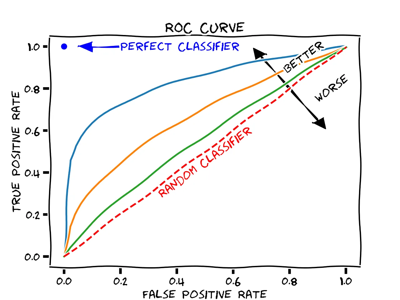
A low threshold means that, even at very low predicted probabilities, we assign “Male” - which means we get most of the males (high True Positive Rate), but we also assign many (true) females to be (false) males (high False Positive Rate). A high threshold means we need a high predicted probability to classify a penguin as male - meaning we err on the side of classifying as female, i.e., a high True Negative Rate - and misclassify many males as females (high False Negative Rate).

Often we don’t even look at the curve, but instead just the area under the curve (AUC) - the ROC curve of a great model will approach the top left of the plot, while a bad model will be close to the diagonal.

To calculate ROC AUC (and the ROC curve) we need not just the predicted classes, but the probabilities associated with the predictions.

peng_prob1 <- peng_assess %>%
  mutate(predict(peng_fit1, new_data = ., type = 'prob'))
yardstick::roc_auc(peng_prob1, truth = sex, .pred_female, event_level = 'first')
yardstick::roc_auc(peng_prob1, truth = sex, .pred_male, event_level = 'second')

peng_prob3 <- peng_assess %>%
  mutate(predict(peng_fit3, new_data = ., type = 'prob'))
yardstick::roc_auc(peng_prob3, truth = sex, .pred_female, event_level = 'first')

1: Here, event_level defines whether we’re looking for the first or second class (female/male in our case), and the .pred_XXX should match the event level.
2: Here we swap for event_level = 'second' and look to .pred_male for our probabilities.

# A tibble: 1 × 3
  .metric .estimator .estimate
  <chr>   <chr>          <dbl>
1 roc_auc binary         0.975
# A tibble: 1 × 3
  .metric .estimator .estimate
  <chr>   <chr>          <dbl>
1 roc_auc binary         0.975
# A tibble: 1 × 3
  .metric .estimator .estimate
  <chr>   <chr>          <dbl>
1 roc_auc binary         0.512

We can also plot the ROC Curve!

roc1_df <- yardstick::roc_curve(peng_prob1, truth = sex, .pred_female)
roc3_df <- yardstick::roc_curve(peng_prob3, truth = sex, .pred_female)

ggplot(data = roc1_df, aes(x = 1 - specificity, y = sensitivity)) +
  geom_abline(intercept = 0, slope = 1, color = 'black') +
  geom_path(color = 'red') +
  geom_path(data = roc3_df, color = 'blue')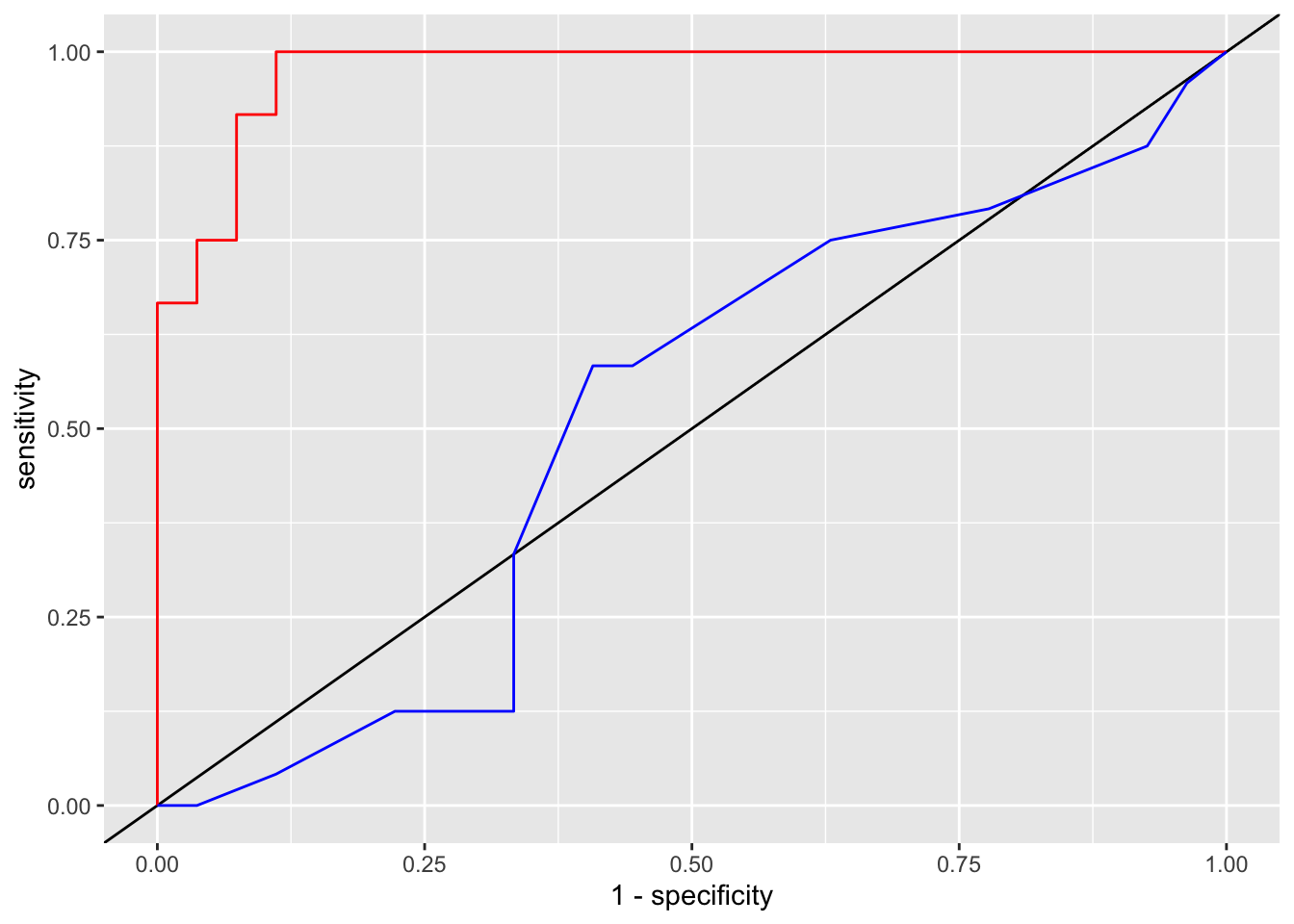

7 Resampling and Cross Validation

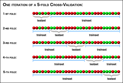
With resampling, we do multiple rounds of partitioning with our training data - iteratively resampling analysis and assessment partitions. Cross validation (CV) is a specific type of resampling - we create multiple equal-sized partitions, called folds, and then set aside one fold as assessment and the remaining folds as analysis to train our data, then use the second fold as assessment etc. If we split our data into five folds we get “five-fold cross validation” - the generic term is K-fold cross validation.

How Many Folds?

Five- and ten-fold CV are basically industry standard - balancing computational effort with accurate performance evaluation, but more art than science. More folds –> less bias, but higher computational cost. Another method, generally only used for small data sets, is n-fold where each observation is its own fold (\(k = N\), also called “Leave-One-Out Cross Validation” (LOOCV) since each iteration leaves out one observation as the assessment set).

Repeated Cross-Validation

Often, after completing one set of cross-validation, we shuffle the observations into a new set of folds and do it all again, iterating many times - “repeated k-fold cross validation”. Repeated CV helps improve consistency of our evaluation metrics – a single round of CV might be prone to an exceptionally lucky (or unlucky) resample, so multiple repeats will help balance that out.

How many repeats? Like folds, choosing a number is more art than science - but ten is a good starting point, and if the model is pretty unstable (high variance from repeat to repeat) 50-100 repeats is not uncommon.

7.1 Cross Validation: Manual Version

For conceptual understanding, five-fold cross validation on our training set peng_train_df might look like this:

Randomly assign each observation to a fold
Set fold 1 aside as assessment, and folds 2-5 as analysis
- Train the desired model on analysis
- Use trained model to predict on assessment
- Calculate some metric of predictive power, e.g., accuracy for classification or RMSE for regression
- Store the metric in a vector
Repeat for the remaining folds

fold_vec <- rep(1:5, length.out = nrow(peng_train_df))
peng_folds_df <- peng_train_df %>%
  mutate(fold = sample(fold_vec, replace = FALSE, size = n()))
  
blm1_results_vec <- rep(NA, 5)

for(i in 1:5) {
  assess_df <- peng_folds_df %>% filter(fold == i)
  analysis_df <- peng_folds_df %>% filter(fold != i)
  
  blm1 <- glm(family = 'binomial', 
              sex ~ species + bill_length_mm + bill_depth_mm, 
              data = analysis_df)
  pred_blm1 <- assess_df %>%
    mutate(prob = predict(blm1, newdata = ., type = 'response'),
           pred_sex = ifelse(prob > 0.5, 'male', 'female'))

  acc_blm1 <- sum(pred_blm1$sex == pred_blm1$pred_sex) / nrow(pred_blm1)
  
  blm1_results_vec[i] <- acc_blm1
}
mean(blm1_results_vec) ### mean accuracy of our given model

1: NOTE: predict() acts differently here than it did earlier, because we are giving it an object of class c('glm', 'lm') - instead of a tidymodels friendly class.

[1] 0.8866541

7.2 Cross Validation with `tidymodels`

Functions from the tidymodels packages automate a lot of that for us. Additionally, we can create a “workflow” that is easy to read and easy to modify/update with new models or even new algorithms.

Resample the data into five folds (v = 5) in a single line - and optionally lets us also do repeated rounds of cross validation (repeats argument) at the same time! Here we only do 3 repeats to keep our examples from being too slow, but 10 would be a better choice.

peng_train_folds <- vfold_cv(peng_train_df, v = 5, repeats = 3)

1: Usually “k-fold cross validation” but tidymodels calls it “v-fold”…?

Now let’s create a workflow (from the workflows package in tidymodels) that combines our model and a formula. We already specified a binary logistic regression model above but we repeat that here for clarity. The workflow specifies how R will operate across all the folds.

blr_mdl <- logistic_reg() %>%
  set_engine('glm')

blr_wf <- workflows::workflow() %>%   ### initialize workflow
  workflows::add_model(blr_mdl) %>%
  workflows::add_formula(sex ~ species + bill_length_mm + bill_depth_mm)

OK now let’s apply the workflow to our folded training dataset (using the fit_resamples function from the tune package in tidymodels), and see how it performs! Note tune::collect_metrics() automatically reports several relevant metrics for the type of model (classification vs. regression).

blr_fit_folds <- blr_wf %>%
  tune::fit_resamples(peng_train_folds)

### Report out the predictive performance across the five folds:
tune::collect_metrics(blr_fit_folds)

# A tibble: 3 × 6
  .metric     .estimator   mean     n std_err .config        
  <chr>       <chr>       <dbl> <int>   <dbl> <chr>          
1 accuracy    binary     0.873     15 0.0124  pre0_mod0_post0
2 brier_class binary     0.0875    15 0.00623 pre0_mod0_post0
3 roc_auc     binary     0.954     15 0.00691 pre0_mod0_post0

8 Model Selection

Our goal with machine learning is to find a model that best predicts our outcome of interest. Typically we have more than one candidate model to consider, including variations on predictors and/or entirely different algorithms. For each candidate model, we can apply the previous steps. Here, we will try several different algorithms and model specifications.

Model specifications
- sex ~ species + bill_length_mm + bill_depth_mm (previous step)
- sex ~ species + bill_length_mm + bill_depth_mm + flipper_length_mm + body_mass_g (all biometrics)
- sex ~ species + island + year (garbage model, for comparison)
Algorithms
- Binomial logistic regression (previous model)
- Random Forest classifier: ensemble of small decision trees
- Support Vector Machine classifier: finds best boundary that separates different groups

8.1 Define Model Specifications

We can create formula objects easily, and give them a short name for easy reference. This is handy to apply a model specification across multiple algorithms. The formula we would normally insert into the model function, we can just assign to a named object. R will not attempt to apply the formula until we call it within the model function.

spec1 <- sex ~ species + bill_length_mm + bill_depth_mm + flipper_length_mm + body_mass_g
spec2 <- sex ~ species + bill_length_mm + bill_depth_mm
spec3 <- sex ~ species + island + year

8.2 Define Model Architecture

Using tidymodels (specifically parsnip package) we can define the model architectures separately from the model specifications. Similar to the model specifications, this is handy to apply different algorithms easily. NOTE: you may need to install the ranger and kernlab packages - the model engines are not included in tidymodels.

blr_mdl <- parsnip::logistic_reg() %>%
  parsnip::set_engine('glm')

rf_mdl <- parsnip::rand_forest(trees = 1000) %>%
  parsnip::set_engine('ranger') %>%
  parsnip::set_mode('classification')
  
svm_mdl <- parsnip::svm_linear() %>%
  parsnip::set_engine('kernlab') %>%
  parsnip::set_mode('classification')

1: We already defined blr_mdl above, repeating here for clarity
2: 'ranger' is the default engine for RF, so technically we don’t need to specify here, but if we wanted to use a different computational engine (e.g., 'randomForest'), we could put that here.
3: Random Forest can be used for classification OR regression; here need to specify which approach we want!
4: The default for svm_linear is LiblineaR but it doesn’t work well with character variables, so here we’ll specify an alternative computational engine from the kernlab package.
5: Similar to random forest, support vector machines can be used for classification OR regression, so we need to specify which.

Computational Engines

Most model algorithms are available from different computational engines, e.g., for logistic regression we could use the glm() implementation, or glmnet, LiblineaR, stan, etc. To see the available engines for an algorithm, use show_engines() with the name of the algorithm function in parsnip, e.g., show_engines('logistic_reg') or show_engines('rand_forest').

8.3 Compare Models

Having defined the model specifications and architectures, let’s create workflows, apply them to our peng_train_folds set, and see the results. Note how little we have to change to test a completely different model!

Here, the workflows are explicitly spelled out one at a time. In the other tabs, we show options for programmatic iteration!

blr_spec1 <- workflow() %>%
  add_model(blr_mdl) %>%
  add_formula(spec1) %>%
  fit_resamples(peng_train_folds)

blr_spec2 <- workflow() %>%
  add_model(blr_mdl) %>%
  add_formula(spec2) %>%
  fit_resamples(peng_train_folds)

blr_spec3 <- workflow() %>%
  add_model(blr_mdl) %>%
  add_formula(spec3) %>%
  fit_resamples(peng_train_folds)

collect_metrics(blr_spec1, type = 'wide')

# A tibble: 1 × 4
  .config         accuracy brier_class roc_auc
  <chr>              <dbl>       <dbl>   <dbl>
1 pre0_mod0_post0    0.915      0.0615   0.976

collect_metrics(blr_spec2, type = 'wide')

# A tibble: 1 × 4
  .config         accuracy brier_class roc_auc
  <chr>              <dbl>       <dbl>   <dbl>
1 pre0_mod0_post0    0.873      0.0875   0.954

collect_metrics(blr_spec3, type = 'wide')

# A tibble: 1 × 4
  .config         accuracy brier_class roc_auc
  <chr>              <dbl>       <dbl>   <dbl>
1 pre0_mod0_post0    0.453       0.261   0.468

Iterate over the specifications using a for loop, printing out the metrics at the end of each iteration.

spec_list <- list(spec1, spec2, spec3)

for(spec in spec_list) {
  rf_specs <- workflow() %>%
    add_model(rf_mdl) %>%
    add_formula(spec) %>%
    fit_resamples(peng_train_folds)
  
  results <- collect_metrics(rf_specs, type = 'wide')
  print(results)
}

# A tibble: 1 × 4
  .config         accuracy brier_class roc_auc
  <chr>              <dbl>       <dbl>   <dbl>
1 pre0_mod0_post0    0.901      0.0752   0.965
# A tibble: 1 × 4
  .config         accuracy brier_class roc_auc
  <chr>              <dbl>       <dbl>   <dbl>
1 pre0_mod0_post0    0.844       0.107   0.939
# A tibble: 1 × 4
  .config         accuracy brier_class roc_auc
  <chr>              <dbl>       <dbl>   <dbl>
1 pre0_mod0_post0    0.415       0.265   0.392

Iterate over the specifications using purrr::map, collecting the metrics across the specs as a list of dataframes, which we then bind together into a single dataframe.

spec_list <- list(spec1, spec2, spec3)

svm_specs <- purrr::map(
  .x = spec_list,
  .f = function(spec) {
    mdl <- workflow() %>%
      add_model(svm_mdl) %>%
      add_formula(spec) %>%
      fit_resamples(peng_train_folds)
    
    collect_metrics(mdl, type = 'wide')
  })

svm_specs_df <- svm_specs %>%
  setNames(as.character(spec_list)) %>%
  bind_rows(.id = 'model_spec')

svm_specs_df

# A tibble: 3 × 5
  model_spec                                .config accuracy brier_class roc_auc
  <chr>                                     <chr>      <dbl>       <dbl>   <dbl>
1 sex ~ species + bill_length_mm + bill_de… pre0_m…    0.920      0.0607   0.975
2 sex ~ species + bill_length_mm + bill_de… pre0_m…    0.873      0.0887   0.954
3 sex ~ species + island + year             pre0_m…    0.472      0.253    0.483

8.4 Results

Across all algorithms, specification 1 (using all available biometric predictors) moderately outperformed specification 2 (with fewer biometric predictors), and specification 3 (with no biometrics) was generally worse than just random guessing.

Across the algorithms, SVM \(\succsim\) Logistic Regression \(\succ\) Random Forest.

Based on these performance evaluation metrics, for our final model let’s use specification 1 with a support vector machine algorithm.

9 Finalizing the Model

At this point, we have partitioned our data using cross validation to identify the best model. Now, we can put in all the training data into our selected model to finalize our model parameters, weights, and coefficients, then compare to the test data we set aside at the very beginning. The function parsnip::last_fit() does all this for us, when we pass it our peng_split object that contains both the peng_train_df and peng_test_df.

### set up our final model as a workflow
final_workflow <- workflow() %>%
  add_model(svm_mdl) %>%
  add_formula(spec1)    ### specification with all biometric variables

final_fit <- last_fit(final_workflow, peng_split)

collect_metrics(final_fit)

# A tibble: 3 × 4
  .metric     .estimator .estimate .config        
  <chr>       <chr>          <dbl> <chr>          
1 accuracy    binary        0.902  pre0_mod0_post0
2 roc_auc     binary        0.966  pre0_mod0_post0
3 brier_class binary        0.0763 pre0_mod0_post0

10 Optional: Recipes for Pre-Processing

For our example, our dataset was already pretty clean and well formed.
recipes: Manages data preprocessing and feature engineering. Use it to define the steps required to clean your data, handle missing values, normalize numeric variables, and encode categorical features.

11 Optional: Model Tuning for Improved Performance

So far we have split our data, used cross validation to identify the best model algorithm and specification, then applied that to our full training data. The tidymodels model functions (logistic_reg, random_forest, svm_linear, etc.) each have several hyperparameters, configuration settings that affect how the model learns from the data. Out of the box, tidymodels assigns sensible values for those hyperparameters, but in some cases, those default values can be tweaked to improve the machine learning performance - particularly to avoid overfitting and underfitting. Model parameters (such as model coefficients and weights) are learned from the data, but hyperparameters control the learning process itself.

Random Forest, for example, has parameters that control the number of decision trees, the number of random features (variables) considered at each node split, tree depth, etc. Support Vector Machines are configured with parameters for kernel (the mathematical function to transform data into higher-dimensional space - linear, polynomial, distance-based methods), and regularization parameter C and gamma parameter \(\gamma\) to trade off between smoother vs. more tightly curving decision boundaries. Other algorithms, including logistic regression, might have hyperparameters to apply penalties or costs to large coefficients or large feature sets.

11.1 Common Model Tuning Algorithms

A grid search tuning algorithm assigns a vector of values to test for each hyperparameter. Across multiple hyperparameters, this creates a multi-dimensional grid or array of possible combinations. Grid search checks every single combination to look for the optimal set. As such, it is intuitive and thorough, but computationally expensive - a brute force approach.

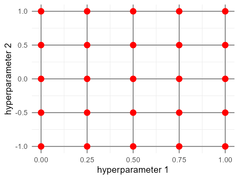
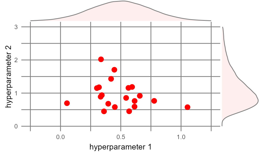
A randomized search tuning algorithm randomly samples many potential combinations of hyperparameters. The values to test for each hyperparameter are drawn from some distribution provided by the user. Unlike grid search, this tuning algorithm concentrates its efforts on regions of each hyperparameter that are most likely according to the given probability distributions, and is generally able to find a good combination faster than a complete grid search. In the example image, test values for hyperparameter 1 are chosen assuming a normal distribution, while values for hyperparameter 2 are chosen from a skewed distribution.

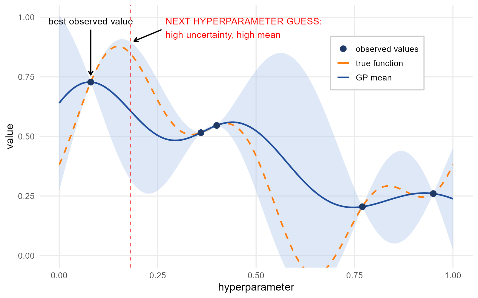
Bayesian optimization tuning algorithm iteratively builds a probabilistic map across hyperparameter space, using a Gaussian process (GP) to approximate the true objective function we want to maximize. To identify likely values to sample, the algorithm focuses on areas of the parameter space with high information value. This balances “exploration” (areas of high uncertainty) against “exploitation” (areas of high expected value). As each point is tested, that information is fed back to the probabilistic model of parameter space, and the next point is chosen to once again maximize the expected information value.

In the example shown (for a single hyperparameter, for simplicity), the black points have already been tested - so uncertainty collapses to zero. A value of ~0.18 falls in a region of high uncertainty (wide confidence interval) and likely high value (GP mean is high). After sampling this point, the confidence intervals and GP mean function will shift accordingly, and the iteration will continue until some stop rule is reached.

11.2 Tuning Model Hyperparameters

Each model type has a different set of hyperparameters with different default values and ranges, which can be found by querying the model function help page (for our purposes, ?svm_linear reveals two parameters, cost and margin).

To prepare for tuning, we redefine our model and set the model’s parameters to a placeholder function tune() to flag it for optimization. Then let’s rebuild our model specification using spec1 from above (the one with all the biometric variables) using the same workflow from before. We will also reuse our folds defined above - peng_train_folds defined with vfold_cv() - for cross validation during the tuning process.

mdl_tune <- svm_linear(cost = tune(), margin = tune()) %>%
  set_engine('kernlab') %>%
  set_mode('classification')

wf_tune <- workflow() %>%
  add_model(mdl_tune) %>%
  add_formula(spec1)

Let’s try Bayesian optimization! (A grid search is already outlined in the tidymodels documentation).

We provide our model specification and our resamples to the tune_bayes() function to identify the best values for our parameters. From these results, we select the best parameter set using the cleverly named function select_best().

bayes_results <- tune_bayes(
  object = wf_tune,
  resamples = peng_train_folds
)

best_params <- select_best(bayes_results, metric = 'roc_auc')

We can insert these best hyperparameter values back into our workflow, and then perform our final fit just as we did above.

final_tuned_wf <- finalize_workflow(wf_tune, best_params)

final_tuned_fit <- last_fit(final_tuned_wf, peng_split)

12 Optional: Model Interpretation

Often we want to know which variables were most influential or important to the predictive power of our Machine Learning model. For a simple linear regression, the magnitude, sign, and p value (or t score) of the coefficients gives us a lot of information about the influence of the variables. For more complex ML models, we generally trade off predictive ability against mechanistic understanding.

To ML or not to ML? Predictive ability vs. scientific insight

Machine learning is often quite amazing at creating predictive models from data, without even needing to know much a priori about the data or ecological system described by the data. If predictions are the important output of an analysis, ML is a great tool

However, we are often more interested in developing insights about the ecological system described by the data. In this case, a structural model that incorporates theoretical underpinnings of the system may be more informative, even if its predictive ability is lower.

Machine learning creates predictive models directly from the data - what will happen. Structural models are informed by expert domain knowledge and theory - why will that happen. Which question are you asking will help determine which approach you should take.

The vip package (“Variable Importance”) combines reasonably well with tidymodels. We can extract our fit information, using tune::extract_fit_parsnip (since our fit is performed using parsnip functions), and then hand this off to the vip::vip() function.

UNfortunately, this doesn’t work well for all model types - e.g., svm_linear models are not well supported (yet?). And for certain models (e.g., random forest with ranger engine), you may need to set parameters in the definition of the model ahead of time. (It can be a bit finicky and model dependent! be patient and Google well!)

To demonstrate, let’s recreate a final fit using our Binomial Logistic Regression model:

final_workflow_blr <- workflow() %>%
  add_model(blr_mdl) %>%
  add_formula(spec1)    ### specification with all biometric variables

final_fit_blr <- last_fit(final_workflow_blr, peng_split)

final_fit_blr %>%
  collect_predictions() %>%
  roc_curve(truth = sex, .pred_male, event_level = 'second') %>%
  autoplot()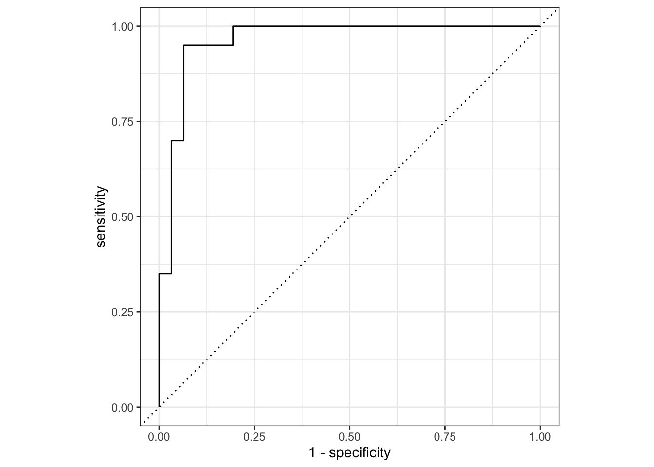

final_fit_blr %>%
  workflows:: extract_fit_parsnip() %>%
  vip::vip()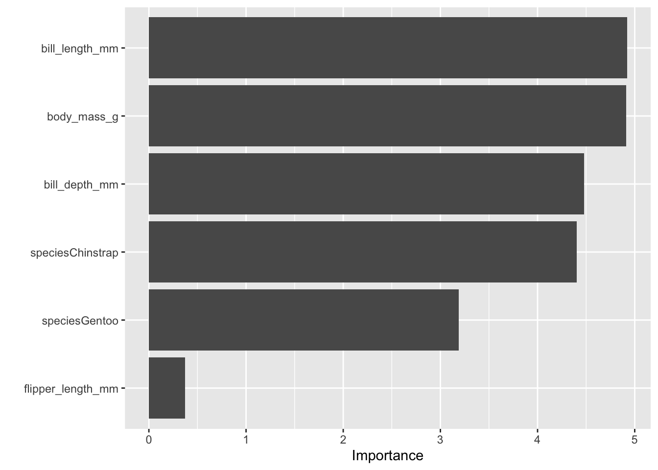

13 Exercise: Create a Regression Model

From the ltersampler R package, load the knz_bison dataset of bison metrics:

Historical records of end-of-season weights for individual bison at Konza Prairie Biological Station LTER.

More information on the dataset here.

For this exercise, we will use the methods above to create and assess several candidate models to predict bison weight based on some combination of variables within the dataset, then select one of the candidate models and determine the performance of the final fit.

data_code: a character denoting the dataset code
rec_year/rec_month/rec_day: a number denoting the year/month/day of observation
animal_code: a character denoting the unique individual bison identification code based on ear tag number
animal_sex: a character denoting the sex of bison: M = male, F = female, U = unknown
animal_weight: a number denoting bison weight in pounds
animal_yob: a number denoting the year animal was born

13.1 Load bison data

library(lterdatasampler)
data(knz_bison) 

# head(knz_bison)
# # A tibble: 6 × 8
# #   data_code rec_year rec_month rec_day animal_code animal_sex animal_weight animal_yob
# #   <chr>        <dbl>     <dbl>   <dbl> <chr>       <chr>              <dbl>      <dbl>
# # 1 CBH01         1994        11       8 813         F                    890       1981
# # 2 CBH01         1994        11       8 834         F                   1074       1983
# # 3 CBH01         1994        11       8 B-301       F                   1060       1983

bison_clean <- knz_bison %>% drop_na()

Hint

These data are NOT linear:

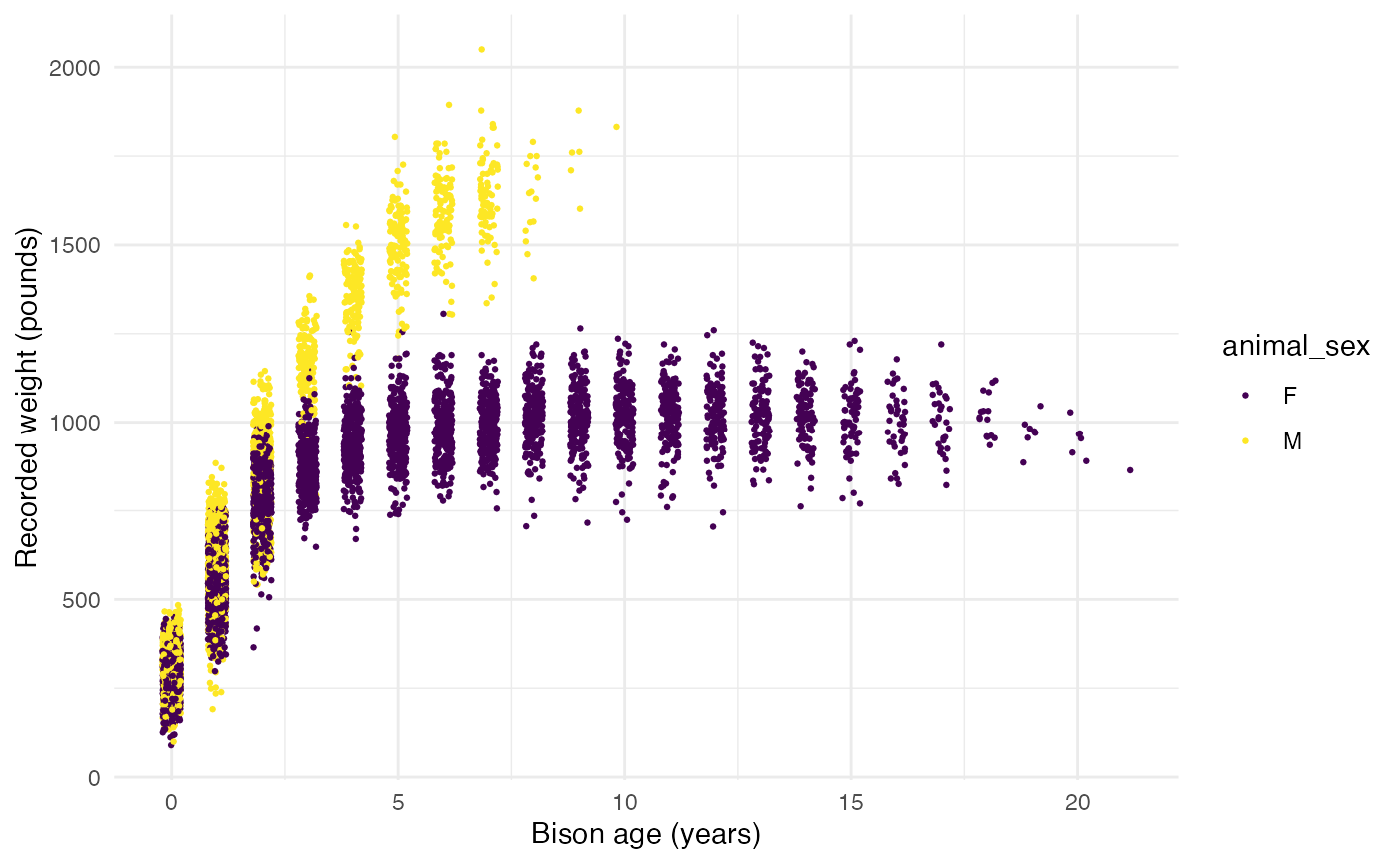
This non-linear data is well suited to non-linear least squares estimation, particularly for an age-growth relationship. But not knowing that relationship, how well can different ML algorithms create predictive models?

We should expect that a linear model will perform poorly, and a linear SVM may similarly struggle. But a good ML algorithm may be able to track non-linearities by learning on the data itself.

Also notable, the Gompertz model is a function of age - and age is not a variable in the dataset! A good ML algorithm may be able to infer age by noting the relationships between animal_weight, animal_yob, and rec_year.

Exercise - Define model specifications

Identify two potentially good model specifications, and one likely very poor specification. Store these specifications as formula objects with names of your choice.

Answer

Your models may vary! Some options:

### Drop animal_code and data_code; all date info
bison_spec1 <- animal_weight ~ rec_year + rec_month + rec_day + animal_sex + animal_yob

### Predict using animal_yob and rec_year (can it identify the age?) and sex
bison_spec2 <- animal_weight ~ rec_year + animal_sex + animal_yob

### Just try sex and the year of birth?
bison_spec3 <- animal_weight ~ animal_sex + animal_yob

Exercise - Define several model architectures

Choose several potential model architectures and define them, including setting an engine. Random Forest and Support Vector machines both can be used for classification (as in the demonstration) and regression (as you might choose to do here!).

Answer

Again, your models may differ - here are some potential options:

bison_lm_mdl <- parsnip::linear_reg() %>%
  parsnip::set_engine('lm')

bison_rf_mdl <- parsnip::rand_forest(trees = 1000) %>%
  parsnip::set_engine('ranger') %>%
  parsnip::set_mode('regression')
  
bison_svm_mdl <- parsnip::svm_linear() %>%
  parsnip::set_engine('kernlab') %>%
  parsnip::set_mode('regression')

1: Classic linear regression instead of binomial logistic - using the base lm engine
2: Set the mode for Random Forest to be regression instead of classification
3: Still using the kernlab engine, but the LiblineaR default may also work - though you may need to install the package!
4: Set the mode to regression, instead of classification

Exercise - Partition data

Partition data into a training and testing set (stratifying if necessary), then set up the training set for cross validation. Choose a number of folds, and a number of repeats if desired.

Answer

You may choose to stratify on site/site name, or date, but the samples are reasonably distributed across those variables. Here’s code that does not stratify the resampling. We choose 10 folds and 5 repeats, though you may choose other options.

bison_split <- initial_split(bison_clean, prop = .85)
bison_train <- training(bison_split)
bison_test   <- testing(bison_split)

bison_folds <- vfold_cv(bison_train, v = 10, repeats = 5)

Exercise - Fit data to models and assess performance

Iterate (manually or programmatically) over the specs and models, fitting the CV folds, then gather the performance metrics to compare results. For iteration, consider a for loop or purrr::map (potentially nesting to iterate over multiple variables).

Answer

Here is an example using purrr::map_df to fit model architectures to each of our model specs, and gather the results as rows in a data frame. First we define a function that takes a model and a spec, and performs the fit then reports metrics.

fit_mdl_spec = function(mdl, spec, folds) {
  fit_result <- workflow() %>%
    add_model(mdl) %>%
    add_formula(spec) %>%
    fit_resamples(folds)
  
  collect_metrics(fit_result, type = 'wide')
}

spec1_results <- purrr::map_df(
  .x = list(bison_lm_mdl, bison_rf_mdl, bison_svm_mdl),
  .f = fit_mdl_spec,
  spec = bison_spec1, folds = bison_folds
)

spec2_results <- purrr::map_df(
  .x = list(bison_lm_mdl, bison_rf_mdl, bison_svm_mdl),
  .f = fit_mdl_spec,
  spec = bison_spec2, folds = bison_folds
)

spec3_results <- purrr::map_df(
  .x = list(bison_lm_mdl, bison_rf_mdl, bison_svm_mdl),
  .f = fit_mdl_spec,
  spec = bison_spec3, folds = bison_folds
)

Spec 1 with a Random Forest does an excellent job of predicting! How well does your model perform?

algorithm	rmse	rsq
Linear regression	243.	0.491
Random forest	122.	0.924
SVM linear	247.	0.478

The RF model on the year/sex/DOB only performed well, R² ~ .76 of the variance, while the model on site and DOB only explained R² ~ 0.12 of the variance.

Exercise - Select a model and perform final fit

From the cross validation results, choose an appropriate model, do a final fit on the full training data, then compare performance against the test set.

Answer

bison_final_wf <- workflow() %>%
  add_model(bison_rf_mdl) %>%
  add_formula(bison_spec1) ### specification with full date, yob, sex

bison_final_fit <- last_fit(bison_final_wf, bison_split)

bison_final_metrics <- collect_metrics(bison_final_fit)
bison_final_preds <- collect_predictions(bison_final_fit)

print(bison_final_metrics)
ggplot(bison_final_preds, aes(x = animal_weight, y = .pred)) +
  geom_point() +
  geom_abline(yintercept = 0, slope = 1, color = 'red') +
  theme_minimal()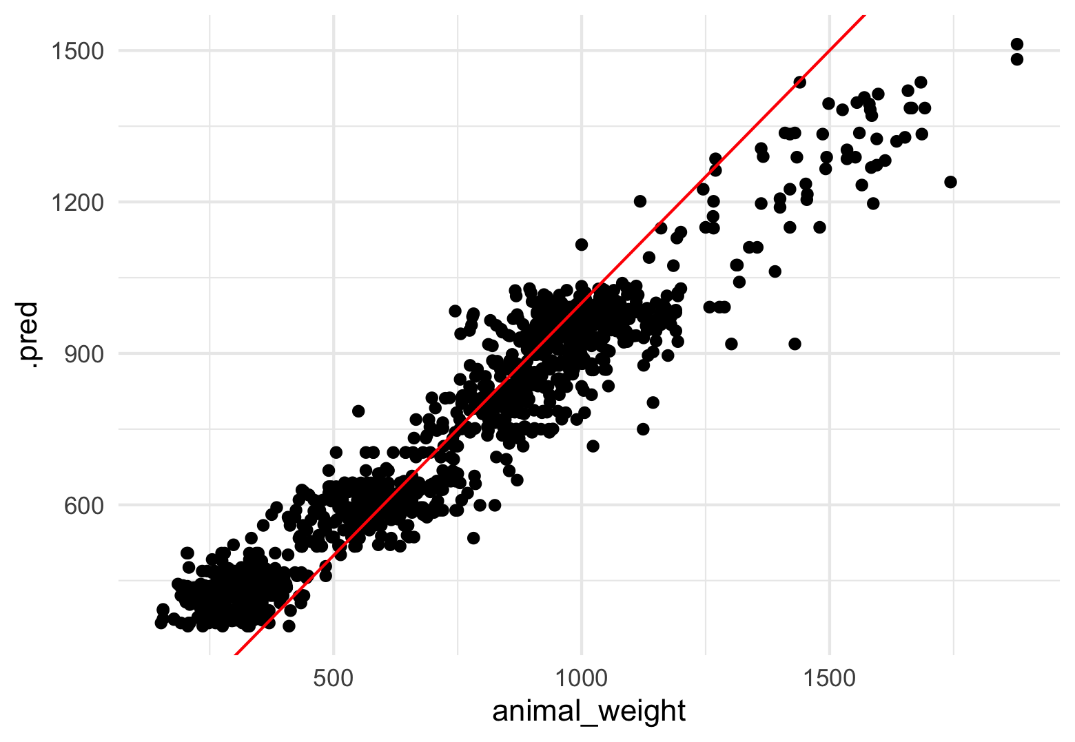

Considering that the weight of the bison is driven primarily by the bison’s age, and age is NOT in the dataset as its own variable, Random Forest does a remarkable job of picking out the patterns based on DOB and year of observation.

1 Overview

2 Machine Learning Overview

3 Setup

3.1 Intro to tidymodels and Component Packages

3.2 Data Overview

3.3 Attach Packages and Load Data

4 Data Partitioning

4.1 Manual Partitioning

4.2 Partitioning With rsample::initial_split

5 Pre-Processing Data with recipes

6 Setting Up A Model

6.1 Assessing Model Performance

7 Resampling and Cross Validation

7.1 Cross Validation: Manual Version

7.2 Cross Validation with tidymodels

8 Model Selection

8.1 Define Model Specifications

8.2 Define Model Architecture

8.3 Compare Models

8.4 Results

9 Finalizing the Model

10 Optional: Recipes for Pre-Processing

11 Optional: Model Tuning for Improved Performance

11.1 Common Model Tuning Algorithms

11.2 Tuning Model Hyperparameters

12 Optional: Model Interpretation

13 Exercise: Create a Regression Model

13.1 Load bison data

3.1 Intro to `tidymodels` and Component Packages

4.2 Partitioning With `rsample::initial_split`

5 Pre-Processing Data with `recipes`

7.2 Cross Validation with `tidymodels`