Shiny is an R package that turns your analyses into interactive web applications, without requiring web development experience. For practicing scientists and managers, this opens up real possibilities: imagine building an app that lets stakeholders explore water quality trends over time, filter fish species occurrence records by season or location, or see how monitoring outcomes compare across management scenarios – all through a browser, with no R knowledge required on their end.
In this session, we’ll build interactive data apps from scratch using water quality and fish catch data from the Yolo Bypass Fish Monitoring Program. By the end of the core session, you’ll have a working reactive Shiny app and the foundation to start building your own for the group projects.
2 What is Shiny?
Shiny is an R package for creating interactive web applications entirely from R code, without needing to learn HTML, JavaScript, or CSS.
Where Shiny fits in the data product landscape
You have multiple choices for how to package up and share your code-driven data analysis and findings. Consider the following table. From top to bottom, each option offers increasing interactivity, but also more complexity:
Product
What it is
Interactivity
Script or notebook
R code + narrative, rendered once
None (static output)
Quarto document
Reproducible report, shareable as HTML or PDF
None (static output)
Quarto doc with widgets
Same, but embeds JS-based widgets
Limited (readers can pan/zoom a Leaflet map, sort a DataTable, or hover over a Plotly chart, but only within pre-rendered data)
Shiny app
Live R process responds to user input
Full (users control what data is shown, what models are run, what is downloaded)
The key distinction: widgets like Leaflet, DataTables, and Plotly are rendered once when the document is generated. They’re clever HTML/JavaScript that runs in the browser with a fixed dataset. In contrast, a Shiny app keeps an R session running on a server, so every user action can trigger new computations, filter different data, or call external APIs.
Why build a Shiny App?
Rationale
Example
Share environmental monitoring data in an engaging, interactive format
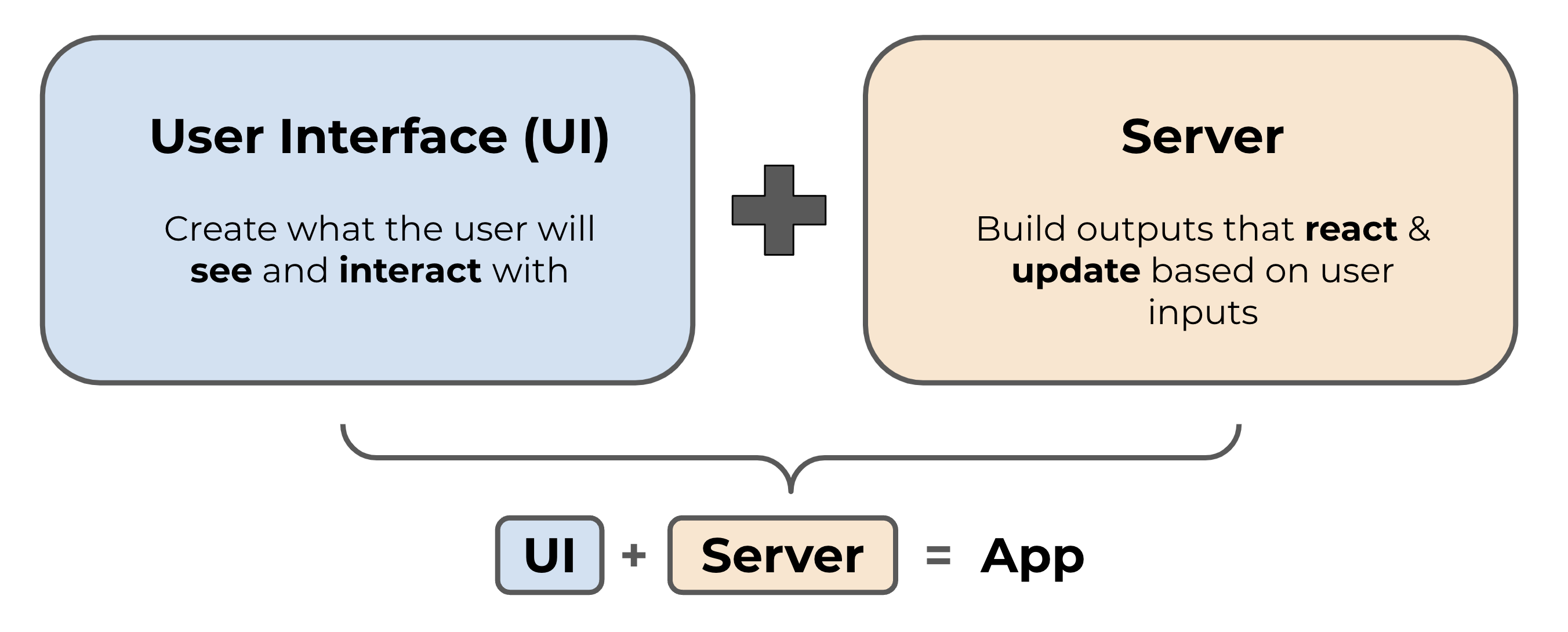
A user interface (UI): the web page your users see and interact with (the “frontend”)
A server function: the R code that powers the app’s computations (the “backend”)
Source: Intro to Shiny - EDS 430, Bren School UCSB
The UI controls layout and appearance. It is written using functions from the {shiny} and {bslib} packages that generate HTML behind the scenes. The server contains the backend logic in the form of instructions for how to respond when a user makes a change.
Here’s what the code for a minimal Shiny app looks like:
library(shiny)library(bslib)### define the UI ui <-page_sidebar(title ="My First App",sidebar =sidebar(),"Hello there!")### define the server ----server <-function(input, output) {}### launch the app ----shinyApp(ui = ui, server = server)
1
page_sidebar() from the {bslib} package creates a modern dashboard-style page with a sidebar and main content area. This is the recommended starting point for most apps.
2
The sidebar() is where user controls (inputs) will live. It’s empty for now.
3
The server is a function with input and output arguments. Even when there’s nothing to compute, it must be defined.
NoteA note on older Shiny code
You may encounter older examples that use fluidPage() + sidebarLayout() for page layout. These still work but are the legacy approach. The {bslib} package – which provides Bootstrap 5-based layouts – is now the recommended way to build Shiny UIs, and is what Posit’s own documentation leads with. We use {bslib} throughout this lesson.
What goes in each section?
Section
Component
UI
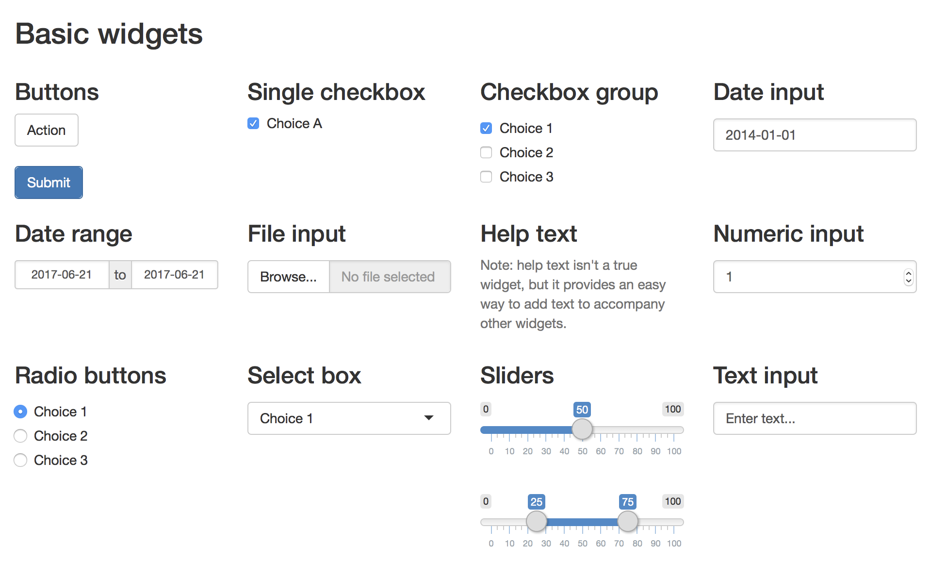
Inputs: widgets that collect values from the user (sliders, dropdowns, checkboxes)
Outputs: placeholders for R objects the user sees (plots, tables, text)
Layout: how components are arranged on the page
Server
Computations: code that creates outputs in response to user inputs
Outputs are R objects displayed in the app. Each type has a matching pair of functions: a placeholder in the UI and a renderer in the server:
UI placeholder
Server renderer
plotOutput()
renderPlot()
tableOutput()
renderTable()
DT::dataTableOutput()
DT::renderDataTable()
textOutput()
renderText()
leafletOutput()
renderLeaflet()
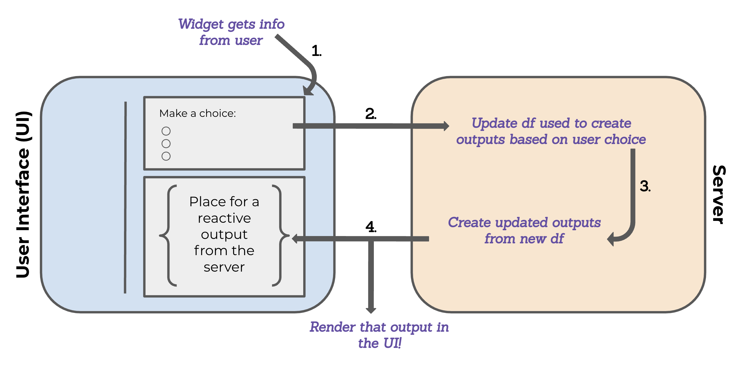
Reactivity: a brief intro
Reactivity is what makes Shiny apps responsive. When a user changes an input value, the server automatically re-runs the relevant code and updates the output. At the most basic level:
Source: Intro to Shiny - EDS 430, Bren School UCSB
Every Shiny app lives in its own folder. The convention is to use a file named app.R for a single-file app, and to house the whole thing in an R Project:
yolo_bypass_app/
├── app.Rthe app!
├── scratch.R for prototyping plots & wrangling (not part of the app)
└── yolo_bypass_app.Rproj project file (if using RStudio)
Create a new folder for your app (e.g., yolo_bypass_app).
In Positron, open the folder as a project: File → Open Folder… and select your folder.
Create a new R file: File → New File → R File and save it as app.R inside your project folder.
Copy the blank app template below into app.R and save.
Run the app by clicking the ▷ Run App button that appears at the top-left of the editor panel (or run shiny::runApp() in the Console).
The app opens in the Viewer pane. To see it in a browser instead, click the Open in Browser icon in the Viewer toolbar.
To stop the app, click the ■ Stop button in the Viewer, or press Escape in the Console.
Create a new project: File → New Project → New Directory → Shiny Application. Name it yolo_bypass_app.
RStudio creates a pre-populated app.R. Replace its contents with the blank template below.
Run the app with the Run App ▷ button at the top-right of the editor.
The app opens in the Viewer pane or a new browser window. Use the dropdown arrow next to Run App to toggle between the two.
To stop the app, click the ■ Stop button in the Viewer, or press Escape in the Console.
### load packages ----library(shiny)library(bslib)### define UI ----ui <-page_sidebar(title ="My App Title",sidebar =sidebar(### inputs will go here"Sidebar widgets will go here" ),### outputs will go here"Output plots will go here")### define server ----server <-function(input, output) {### computations will go here}### launch the app ----shinyApp(ui = ui, server = server)
TipTip: Use code sections for navigation
Code sections (denoted above by ### section name ----) appear as collapsible entries in Positron’s Outline panel and RStudio’s Document Outline, making large app.R files much easier to navigate. Just end any comment line with at least four dashes (----), equals signs (====), or pound signs (####).
TipTip: Add placeholder text and run early
Put placeholder strings, e.g., "Output plots will go here" in this basic template, inside each UI element/section so you can see the structure as you build. Run the app after each addition. Catching errors early saves a lot of debugging time!
5 Building a Reactive App
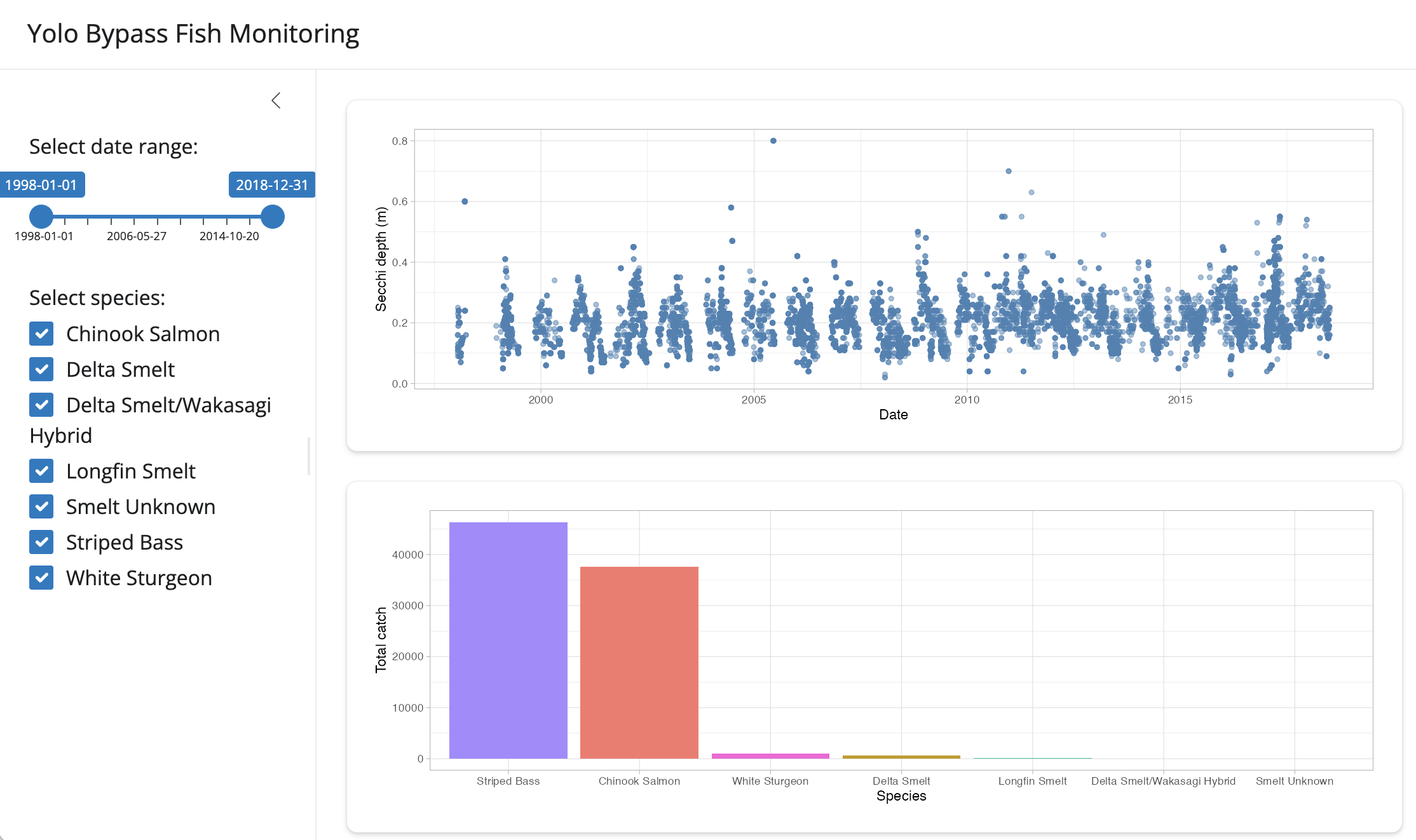
We’ll build an interactive explorer for the Yolo Bypass Fish Monitoring Program dataset, consisting of fish catch and water quality data from the Sacramento River floodplain collected since 1998. The final app will let users filter by date range and explore water clarity trends and fish catch patterns.
Load the data
TipTip: Prototype outside the app first
It’s always easier to develop and test your data loading and plotting code in a regular R script before moving it into the Shiny app. Create a scratch.R file in your app folder for this purpose. Experiment there, then copy working code into app.R.
We’ll use a URL to load the data reliably from the EDI data repository, and do some light data wrangling to turn the SampleDate column into a date format and filter for just a few key fish species.
### load packages ----library(shiny)library(bslib)library(dplyr)library(lubridate)library(ggplot2)### load Yolo Bypass monitoring data from EDI ----delta_file <-"https://pasta.lternet.edu/package/data/eml/edi/233/2/015e494911cf35c90089ced5a3127334"delta_data <-read.csv(delta_file) |>mutate(SampleDate =mdy(SampleDate)) |>filter(grepl("Salmon|Striped Bass|Smelt|Sturgeon", CommonName))### define UI ----ui <-page_sidebar(...)
1
Throughout this lesson we use the base pipe |> which requires R 4.1 or later, though the tidyverse pipe %>% would work too.
Put this data-loading code at the top of app.R, before the ui and server definitions. Code at the top level of app.R (outside ui and server) runs once when the app starts and is available throughout.
TipAccessing data for Shiny
Here we are loading data directly from a URL, but just as for any analysis, you could also save data locally or use programmatic methods for accessing your data from a remote source, e.g., through an API or R package such as contentid.
Step 1: Add a date range slider
We’ll add a sliderInput() inside sidebar() (and update our title):
ui <-page_sidebar(title ="Yolo Bypass Fish Monitoring", sidebar =sidebar(### date range slider ----sliderInput(inputId ="date_range",label ="Select date range:",min =as.Date("1998-01-01"),max =as.Date("2018-12-31"),value =c(as.Date("1998-01-01"), as.Date("2018-12-31")) ) ),### outputs will go here"Output plots will go here")
1
The inputId is how you’ll refer to this input’s current value in the server. Keep it short and descriptive, and remember that spelling matters and it’s case sensitive!
Step 2: Add a plot output placeholder
Output functions in the UI create placeholders. These are slots where server-generated content will appear. We’ll add a plotOutput() inside a card() (replacing our “output plot” text):
ui <-page_sidebar(title ="Yolo Bypass Fish Monitoring",sidebar =sidebar(### date range slider ----sliderInput(inputId ="date_range",label ="Select date range:",min =as.Date("1998-01-01"),max =as.Date("2018-12-31"),value =c(as.Date("1998-01-01"), as.Date("2018-12-31")) ) ), ### END sidebar### Secchi depth plot ----card(plotOutput(outputId ="secchi_plot") )) ### END page_sidebar
1
Comment to flag the closing parenthesis of a major UI element - helpful for reading code now and debugging later!
2
The outputId is quoted in the UI. In the server, you’ll refer to it as output$secchi_plot (unquoted, with $). These must match exactly.
3
Another comment to flag the closing parenthesis of a major UI element.
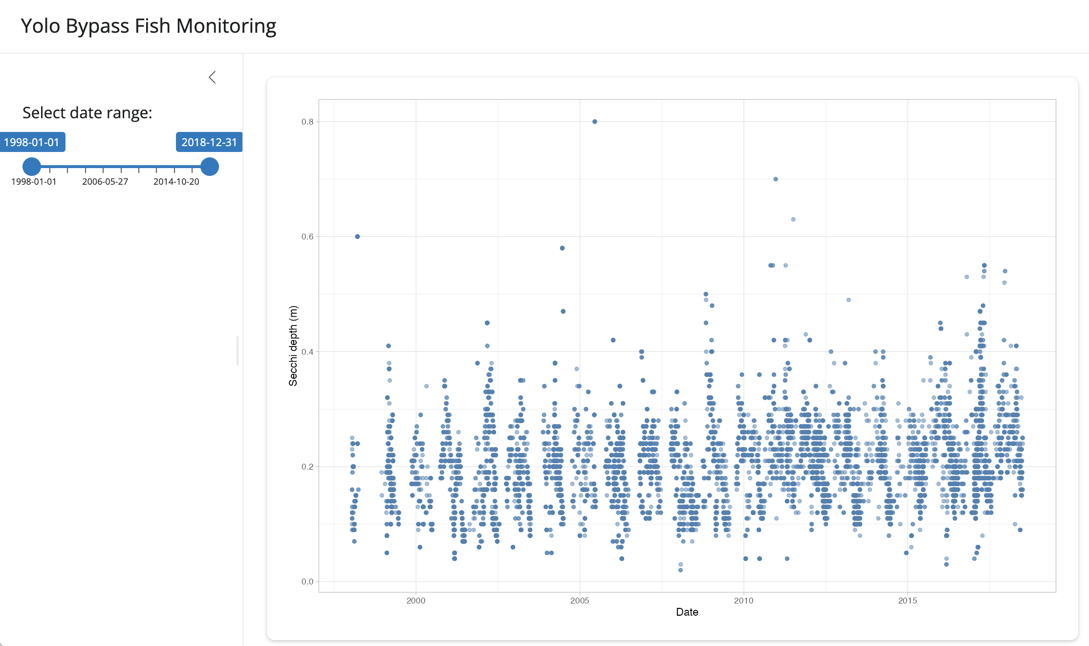
Run the app now. The slider appears, but no plot yet. The placeholder exists, but we haven’t told the server what to put in it.
TipComment Your Closing Parentheses
The UI is a heavily nested structure. To keep track of where one element ends and another begins, add comment lines after the closing parentheses for major UI structure elements, e.g., ### END sidebar and ### END page_sidebar in the example above. (You could also add ### END slider_input though it’s easier to see the structure of that).
These closing notes will be immensely helpful when it’s time for troubleshooting!
Step 3: Tell the server how to create the output
There are three rules for building reactive outputs:
ImportantThe Three Rules of Shiny Reactivity
Rule 1: Save objects you want to display to output$<id>
Rule 2: Build reactive objects using a render*() function
Rule 3: Access input values with input$<id>
Rule 1: Save to output$<id>
server <-function(input, output) { output$secchi_plot <-### plot code goes here}
Rule 2: Build with render*()
Each *Output() UI function is paired with a render*() server function. Because we used plotOutput(), we use renderPlot():
server <-function(input, output) {### render Secchi depth plot ---- output$secchi_plot <-renderPlot({ggplot(delta_data, aes(x = SampleDate, y = Secchi)) +geom_point(color ="steelblue", alpha =0.5) +labs(x ="Date", y ="Secchi depth (m)") +theme_light() })}
Run the app. You now see a plot! But dragging the date slider still doesn’t change anything, because we haven’t connected the slider value to the plot yet.
Rule 3: Access inputs with input$<id>
To make the plot respond to the slider, we filter the data based on the slider’s current value. Because this filtered dataset needs to re-compute every time the slider changes, we wrap it in a reactive() expression.
ImportantReactive expressions and the () requirement
reactive({...}) creates an expression that re-runs automatically whenever any input$ values it depends on change. Whenever you use a reactive expression elsewhere in your server code, you must call it with parentheses: filtered_data(), not filtered_data. This tells Shiny to read the current reactive value.
server <-function(input, output) {### filter data by date range ---- filtered_data <-reactive({ delta_data |>filter( SampleDate >= input$date_range[1], SampleDate <= input$date_range[2] ) })### render Secchi depth plot ---- output$secchi_plot <-renderPlot({ggplot(filtered_data(), aes(x = SampleDate, y = Secchi)) +geom_point(color ="steelblue", alpha =0.5) +labs(x ="Date", y ="Secchi depth (m)") +theme_light() })}
1
reactive({...}) wraps code that should re-run when inputs change
2
input$date_range[1] and [2] are the minimum and maximum of the range slider
3
Note the parentheses: filtered_data() – this is required when calling a reactive expression
Run the app and drag the slider. The plot should now update reactively!
The complete single-file app
Show complete app.R
### load packages ----library(shiny)library(bslib)library(dplyr)library(lubridate)library(ggplot2)### load Yolo Bypass monitoring data from EDI ----delta_file <-"https://pasta.lternet.edu/package/data/eml/edi/233/2/015e494911cf35c90089ced5a3127334"delta_data <-read.csv(delta_file) |>mutate(SampleDate =mdy(SampleDate)) |>filter(grepl("Salmon|Striped Bass|Smelt|Sturgeon", CommonName))### define UI ----ui <-page_sidebar(title ="Yolo Bypass Fish Monitoring",sidebar =sidebar(### date range slider ----sliderInput(inputId ="date_range",label ="Select date range:",min =as.Date("1998-01-01"),max =as.Date("2018-12-31"),value =c(as.Date("1998-01-01"), as.Date("2018-12-31")) ) ), ### END sidebar### Secchi depth plot ----card(plotOutput(outputId ="secchi_plot") )) ### END page_sidebar### define server ----server <-function(input, output) {### filter data by date range ---- filtered_data <-reactive({ delta_data |>filter( SampleDate >= input$date_range[1], SampleDate <= input$date_range[2] ) })### render Secchi depth plot ---- output$secchi_plot <-renderPlot({ggplot(filtered_data(), aes(x = SampleDate, y = Secchi)) +geom_point(color ="steelblue", alpha =0.5) +labs(x ="Date", y ="Secchi depth (m)") +theme_light() })}### launch the app ----shinyApp(ui = ui, server = server)
ImportantCommon mistakes
Misspelling inputId as inputID (or outputId as outputID) – R is case-sensitive.
Mismatched IDs between UI and server (e.g., "secchi_plot" in UI but secchiPlot in server)
Forgetting to separate UI elements with a comma , – nearly every element inside page_sidebar(), sidebar(), or card() needs a comma after it
Forgetting parentheses when calling a reactive expression (e.g., filtered_data should be filtered_data())
Using input$ values outside a reactive context – they can only be read inside reactive(), render*(), or observe()
6 Your Turn: Add a Species Filter
NoteExercise: Add a species checkbox and fish catch plot
Working individually or in pairs, extend your single-file app by adding:
A checkboxGroupInput in the sidebar that lets users select which fish species to display, with all species pre-selected by default
A second card() in the main area containing a plotOutput showing a bar chart of total fish catch by species for the currently selected date range and species
The date range slider and species checkbox should both filter the same reactive dataset.
TipTips
Use ?checkboxGroupInput to see the required arguments (inputId, label, choices, selected)
Get the actual species names with sort(unique(delta_data$CommonName)) – run this in your scratch script first
Prototype the bar chart in scratch.R before adding it to the server: ggplot(data, aes(x = CommonName, y = Count)) + geom_col()
Update your existing filtered_data reactive to also filter by CommonName %in% input$species_select, allowing both plots to share the same filtered data
To get total catch by species: group_by(CommonName) |> summarize(total = sum(Count, na.rm = TRUE))
Solution
### load packages ----library(shiny)library(bslib)library(dplyr)library(lubridate)library(ggplot2)### load Yolo Bypass monitoring data from EDI ----delta_file <-"https://pasta.lternet.edu/package/data/eml/edi/233/2/015e494911cf35c90089ced5a3127334"delta_data <-read.csv(delta_file) |>mutate(SampleDate =mdy(SampleDate)) |>filter(grepl("Salmon|Striped Bass|Smelt|Sturgeon", CommonName))species_choices <-sort(unique(delta_data$CommonName))### define UI ----ui <-page_sidebar(title ="Yolo Bypass Fish Monitoring",sidebar =sidebar(### date range slider ----sliderInput(inputId ="date_range",label ="Select date range:",min =as.Date("1998-01-01"),max =as.Date("2018-12-31"),value =c(as.Date("1998-01-01"), as.Date("2018-12-31")) ),### species checkbox ----checkboxGroupInput(inputId ="species_select",label ="Select species:",choices = species_choices,selected = species_choices ) ), ### END sidebar### Secchi depth plot ----card(plotOutput(outputId ="secchi_plot") ),### fish catch bar chart ----card(plotOutput(outputId ="catch_plot") )) ### END page_sidebar### define server ----server <-function(input, output) {### filter data by date range and species ---- filtered_data <-reactive({ delta_data |>filter( SampleDate >= input$date_range[1], SampleDate <= input$date_range[2], CommonName %in% input$species_select ) })### render Secchi depth plot ---- output$secchi_plot <-renderPlot({ggplot(filtered_data(), aes(x = SampleDate, y = Secchi)) +geom_point(color ="steelblue", alpha =0.5) +labs(x ="Date", y ="Secchi depth (m)") +theme_light() })### render fish catch bar chart ---- output$catch_plot <-renderPlot({filtered_data() |>group_by(CommonName) |>summarize(total_catch =sum(Count, na.rm =TRUE), .groups ="drop") |>ggplot(aes(x =reorder(CommonName, -total_catch),y = total_catch,fill = CommonName)) +geom_col(show.legend =FALSE) +labs(x ="Species", y ="Total catch") +theme_light() })}### launch the app ----shinyApp(ui = ui, server = server)
7 Organizing Your App
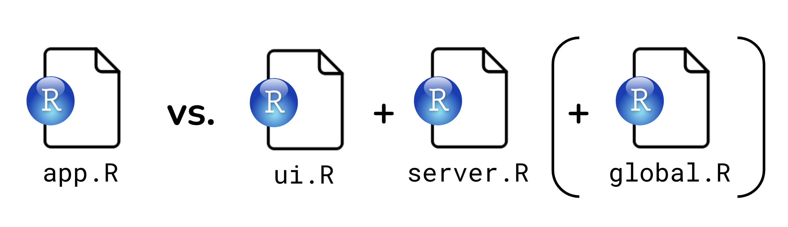
Single-File vs Two-File
So far we’ve put everything in one app.R. For simple apps, this works well. As apps grow, splitting the code into separate files makes it easier to navigate, maintain, and collaborate on.
Source: Intro to Shiny - EDS 430, Bren School UCSB
A third optional file, global.R, runs once before ui.R and server.R (or before app.R for a single-file app). It’s the right place for packages, data loading, and any objects that both files need - in the single-file app above, everything before starting the ui definition is a good candidate for global.R.
Recommended project structure
yolo_bypass_app/
├── global.R(optional) packages + data (runs first, available everywhere)
├── ui.Ruser interface definition
├── server.Rserver logic
├── text/ (optional) text elements for UI
│ └── about.md markdown text for the About page
├── data/ (optional) data for use in app
│ └── my_data.csv
├── www/ (optional) images, HTML, CSS, etc - MUST BE CALLED www!
│ ├── my_styles.css
│ └── my_image.png
├── scratch.R development scratch work (not part of the app)
└── yolo_bypass_app.Rproj project file (if using RStudio)
ImportantThe optional www folder is special!
The optional www folder MUST be called www - this is where Shiny looks for static elements to be rendered in the app, but that are not products of the scripts, like images. When you add an image to your app, you skip the www part in the file path - e.g., img(src = 'my_image.png').
Other folders, e.g., data and text above, can contain files accessed by server.R through regular file path functions, e.g., here::here() or file.path().
8 Building a Two-File App
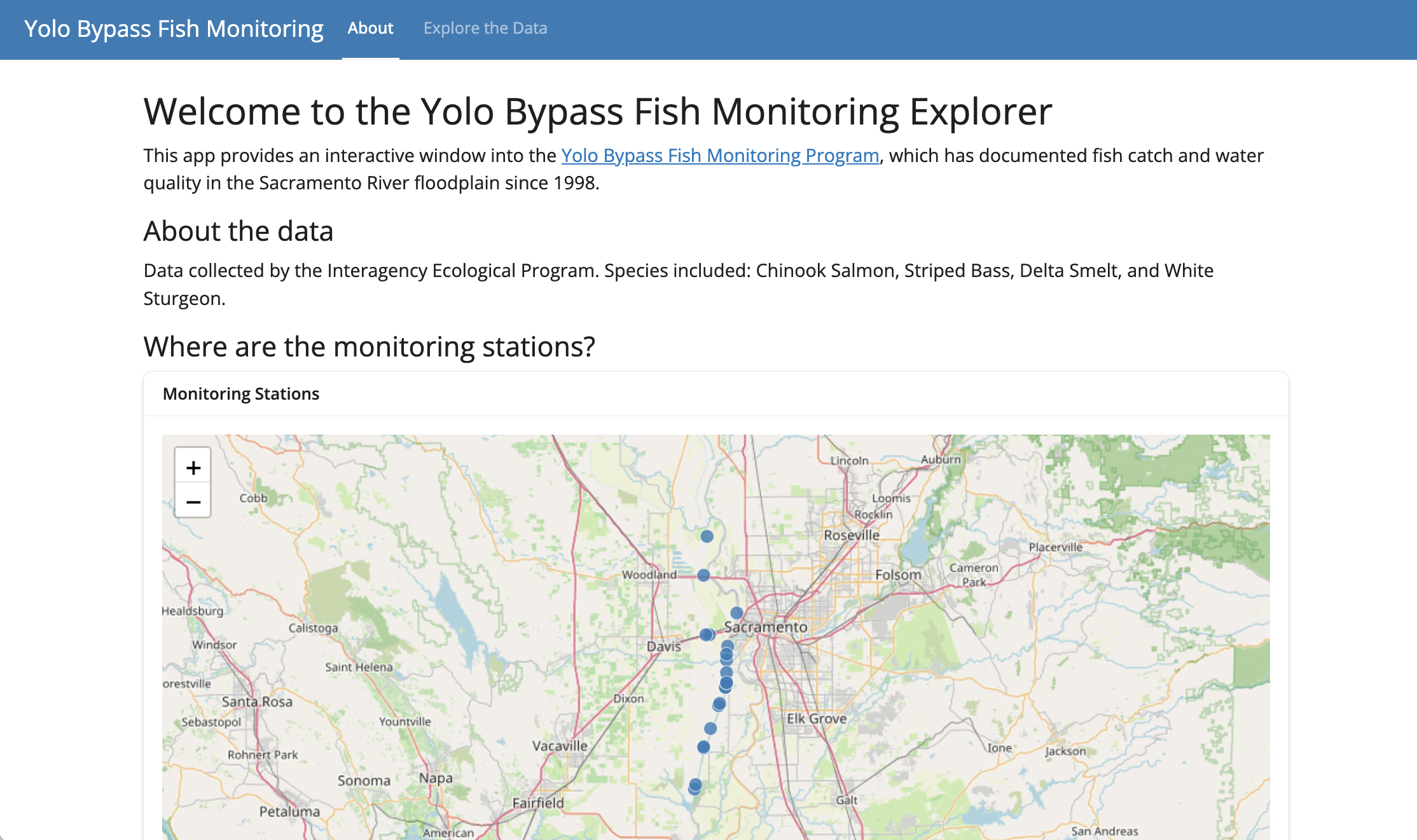
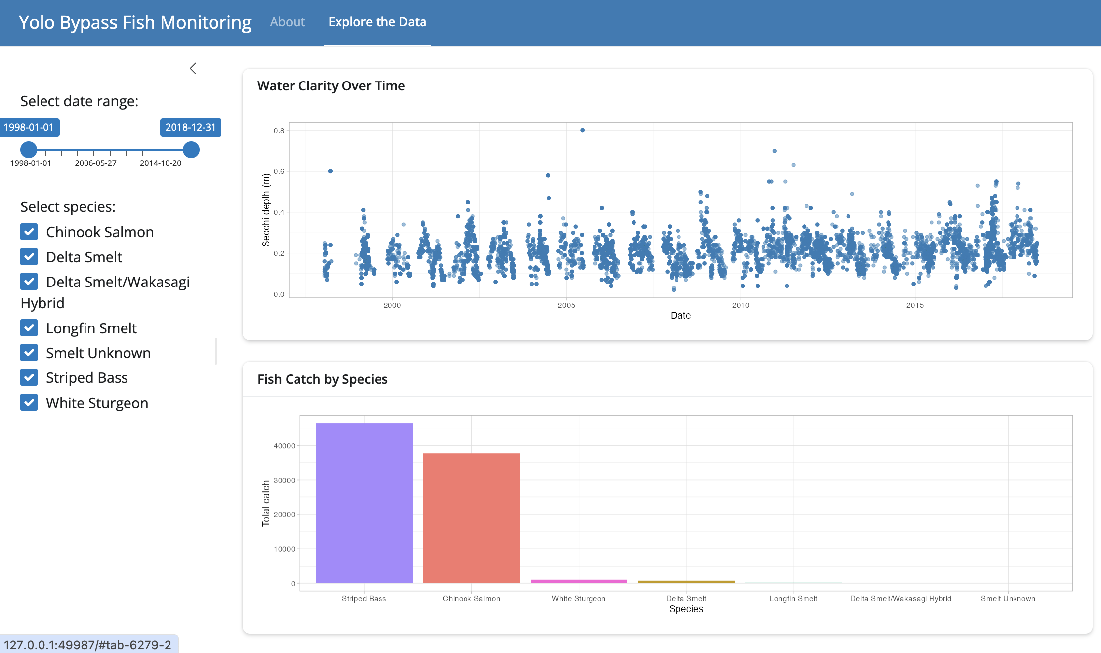
Let’s rebuild the Yolo Bypass app in two-file format with a polished multi-page layout. The finished app will have two pages accessible via a navigation bar: an About page with context and a map, and an Explore page with the interactive plots.
Below includes all the same information we used in the single-file app above, plus station locations we’ll use to expand upon the simple one-file app.
### global.R ----### load packages ----library(shiny)library(bslib)library(dplyr)library(lubridate)library(ggplot2)library(DT)library(leaflet)library(markdown)### load Yolo Bypass monitoring data from EDI ----delta_file <-"https://pasta.lternet.edu/package/data/eml/edi/233/2/015e494911cf35c90089ced5a3127334"delta_data <-read.csv(delta_file) |>mutate(SampleDate =mdy(SampleDate)) |>filter(grepl("Salmon|Striped Bass|Smelt|Sturgeon", CommonName))species_choices <-sort(unique(delta_data$CommonName))### station locations for map ----sites <- delta_data |>distinct(StationCode, Latitude, Longitude) |>drop_na()
8.1 Write UI in ui.R
Here we structure the user interface as a page_navbar() design, with a top navigation bar to navigate among two tabs. We’ll use a few new UI elements to compare to the ones we used in the single-file app.R.
For our “Explore” tab, we’ll add input widgets and outputs that will be generated by our server.R.
For our “About” page we will put the text in a separate Markdown document to make the ui.R a little cleaner, and make it easy to find and update our “About” information without needing to mess with the ui.R file.
page_navbar() creates a full-page layout with a top navigation bar, and nav_panel() defines each tab:
### ui.R ----ui <-page_navbar(title ="Yolo Bypass Fish Monitoring",bg ="#2C7BB6", ### navbar color (hex or named color)### (Tab 1) About ----nav_panel(title ="About",### content will go here ), ### END About tab nav_panel### (Tab 2) Explore the Data ----nav_panel(title ="Explore the Data",### content will go here ) ### END Explore tab nav_panel) ### END page_navbar
Inside “Explore the Data”, we’ll use layout_sidebar() to pair inputs with outputs. Since the date slider affects both plots and the species checkbox also affects both, we use one sidebar for all inputs and two card() outputs in the main area:
ui <-page_navbar( ...### (Tab 1) About ----nav_panel( ... ), ### END About tab nav_panel### (Tab 2) Explore the Data ----nav_panel(title ="Explore the Data",layout_sidebar(sidebar =sidebar(### date range slider ----sliderInput(inputId ="date_range",label ="Select date range:",min =as.Date("1998-01-01"),max =as.Date("2018-12-31"),value =c(as.Date("1998-01-01"), as.Date("2018-12-31")) ),### species checkbox ----checkboxGroupInput(inputId ="species_select",label ="Select species:",choices = species_choices, ### defined in global.Rselected = species_choices ) ), ### END sidebar### Secchi depth plot ----card(card_header("Water Clarity Over Time"),plotOutput(outputId ="secchi_plot") ),### fish catch bar chart ----card(card_header("Fish Catch by Species"),plotOutput(outputId ="catch_plot") ) ) ### END layout_sidebar ) ### END Explore tab nav_panel) ### END page_navbar
For longer descriptive text, write it in a Markdown file and pull it in with includeMarkdown(). Create text/about.md in your app folder:
## Welcome to the Yolo Bypass Fish Monitoring ExplorerThis app provides an interactive window into the [Yolo Bypass Fish Monitoring Program](https://doi.org/10.6073/pasta/b0b15aef7f3b52d2c5adc10004c05a6f),which has documented fish catch and water quality in the Sacramento River floodplainsince 1998.#### About the dataData collected by the Interagency Ecological Program. Species included: Chinook Salmon,Striped Bass, Delta Smelt, and White Sturgeon.#### Where are the monitoring stations?
Then in ui.R, pull it into the About tab alongside a map of station locations:
ui <-page_navbar( ...### (Tab 1) About ----nav_panel(title ="About",layout_columns(col_widths =c(-1, 10, -1),div(includeMarkdown("text/about.md"),card(card_header("Monitoring Stations"),leafletOutput(outputId ="stations_map") ) ) ) ### END layout_columns ), ### END About tab nav_panel### (Tab 2) Explore the Data ----nav_panel( ... ) ### END Explore tab nav_panel) ### END page_navbar
1
col_widths = c(-1, 10, -1) creates 1-column empty gutters on each side and puts the content in the middle 10 of 12 Bootstrap columns, for a clean centered layout.
Write Reactive Functionality in server.R
### server.R ----server <-function(input, output) {### render station locations map ---- output$stations_map <-renderLeaflet({leaflet(sites) |>addTiles() |>addCircleMarkers(lat =~Latitude,lng =~Longitude,radius =6,fillColor ="#2C7BB6",fillOpacity =0.8,weight =1,color ="white",label =~StationCode ) })### filter data by date range and species ---- filtered_data <-reactive({ delta_data |>filter( SampleDate >= input$date_range[1], SampleDate <= input$date_range[2], CommonName %in% input$species_select ) })### render Secchi depth plot ---- output$secchi_plot <-renderPlot({ggplot(filtered_data(), aes(x = SampleDate, y = Secchi)) +geom_point(color ="#2C7BB6", alpha =0.5) +labs(x ="Date", y ="Secchi depth (m)") +theme_light() })### render fish catch bar chart ---- output$catch_plot <-renderPlot({filtered_data() |>group_by(CommonName) |>summarize(total_catch =sum(Count, na.rm =TRUE), .groups ="drop") |>ggplot(aes(x =reorder(CommonName, -total_catch),y = total_catch,fill = CommonName)) +geom_col(show.legend =FALSE) +labs(x ="Species", y ="Total catch") +theme_light() })} ### END server
1
The station map doesn’t depend on any user inputs, so it doesn’t need reactive(). However, it still must be assigned to output$ and wrapped in render*().
### global.R ----### load packages ----library(shiny)library(bslib)library(dplyr)library(lubridate)library(ggplot2)library(leaflet)library(markdown)### load Yolo Bypass monitoring data from EDI ----delta_file <-"https://pasta.lternet.edu/package/data/eml/edi/233/2/015e494911cf35c90089ced5a3127334"delta_data <-read.csv(delta_file) |>mutate(SampleDate =mdy(SampleDate)) |>filter(grepl("Salmon|Striped Bass|Smelt|Sturgeon", CommonName))species_choices <-sort(unique(delta_data$CommonName))### station locations for map ----sites <- delta_data |>distinct(StationCode, Latitude, Longitude) |>drop_na()
Show complete ui.R
### ui.R ----ui <-page_navbar(title ="Yolo Bypass Fish Monitoring",bg ="#2C7BB6",### (Tab 1) About ----nav_panel(title ="About",layout_columns(col_widths =c(-1, 10, -1),div(includeMarkdown("text/about.md"),card(card_header("Monitoring Stations"),leafletOutput(outputId ="stations_map") ) ) ) ), ### END About tab nav_panel### (Tab 2) Explore the Data ----nav_panel(title ="Explore the Data",layout_sidebar(sidebar =sidebar(sliderInput(inputId ="date_range",label ="Select date range:",min =as.Date("1998-01-01"),max =as.Date("2018-12-31"),value =c(as.Date("1998-01-01"), as.Date("2018-12-31")) ),checkboxGroupInput(inputId ="species_select",label ="Select species:",choices = species_choices,selected = species_choices ) ), ### END sidebarcard(card_header("Water Clarity Over Time"),plotOutput(outputId ="secchi_plot") ),card(card_header("Fish Catch by Species"),plotOutput(outputId ="catch_plot") ) ) ### END layout_sidebar ) ### END Explore tab nav_panel) ### END page_navbar
Show complete server.R
### server.R ----server <-function(input, output) {### render station locations map ---- output$stations_map <-renderLeaflet({leaflet(sites) |>addTiles() |>addCircleMarkers(lat =~Latitude,lng =~Longitude,radius =6,fillColor ="#2C7BB6",fillOpacity =0.8,weight =1,color ="white",label =~StationCode ) })### filter data by date range and species ---- filtered_data <-reactive({ delta_data |>filter( SampleDate >= input$date_range[1], SampleDate <= input$date_range[2], CommonName %in% input$species_select ) })### render Secchi depth plot ---- output$secchi_plot <-renderPlot({ggplot(filtered_data(), aes(x = SampleDate, y = Secchi)) +geom_point(color ="#2C7BB6", alpha =0.5) +labs(x ="Date", y ="Secchi depth (m)") +theme_light() })### render fish catch bar chart ---- output$catch_plot <-renderPlot({filtered_data() |>group_by(CommonName) |>summarize(total_catch =sum(Count, na.rm =TRUE), .groups ="drop") |>ggplot(aes(x =reorder(CommonName, -total_catch),y = total_catch,fill = CommonName)) +geom_col(show.legend =FALSE) +labs(x ="Species", y ="Total catch") +theme_light() })} ### END server
## Welcome to the Yolo Bypass Fish Monitoring ExplorerThis app provides an interactive window into the[Yolo Bypass Fish Monitoring Program](https://doi.org/10.6073/pasta/b0b15aef7f3b52d2c5adc10004c05a6f),which has documented fish catch and water quality in the Sacramento River floodplainand tidal slough since 1998.#### About the dataData collected by the Interagency Ecological Program as part of a long-termmonitoring effort in the Yolo Bypass, a critical floodplain habitat for theSacramento-San Joaquin Delta ecosystem. Species monitored include Chinook Salmon,Striped Bass, Delta Smelt, and White Sturgeon.#### Where are the monitoring stations?
9 Sharing Your App
Once you’ve built something worth sharing, there are several ways to get it in front of others:
shinyapps.io is the easiest hosting option. This cloud service provided by Posit has a free tier (up to 5 apps, 25 active hours/month) and paid tiers for more demanding apps.
Click the Publish icon (cloud with arrow) in the Viewer pane toolbar after running your app, or run rsconnect::deployApp("path/to/your/app") directly in the Console.
Click the blue Publish button (cloud icon) in the top-right corner of the running app window, or run rsconnect::deployApp("path/to/your/app") directly in the Console.
shinylive is a newer option that runs Shiny apps entirely in the browser using WebR. No server required! This means:
No hosting costs, because apps can live as static files on GitHub Pages or any web server
Works inside Quarto documents, allowing you to embed an interactive app directly in a .qmd file
Great for teaching and sharing reproducible examples
install.packages("shinylive")### export app (located at `appdir`) to a self-contained static site in ### a new, separate repository (located at `destdir`)shinylive::export(appdir ="yolo_bypass_app/", destdir ="site/")
You can open the site locally, or host it on GitHub Pages or the like.
TipShinylive in Quarto
You can embed Shiny apps directly in Quarto documents using the shinylive Quarto extension. See posit-dev.github.io/r-shinylive for instructions.
NoteLimitations of shinylive
Because apps run in the browser, startup is slower than server-based apps, and some R packages are not yet supported. Best suited for moderately complex apps with typical CRAN packages.
Posit Connect is an enterprise, on-premises product for organizations that need more than shinyapps.io provides. This includes user authentication, scheduled content, and greater control over infrastructure. It’s the right choice for production-grade agency tools.
Wrapping your Shiny app into an R package can allow others to easily install your app from CRAN or from GitHub, and then run it locally. It also provides a more formal structure, formalized documentation, and testing/checking processes. For more information, see this chapter in Mastering Shiny by Hadley Wickham.