# This path only works on one specific machine
delta_catch <- read_csv("C:/Users/jsmith/Documents/2023/delta_catch.csv")

# Relative paths help, but only if the data travels with the code
delta_taxa <- read_csv("../../data_archive/delta_taxa.csv")1 Overview
One of the most common reproducibility barriers in data-driven science isn’t in the analysis code itself, but rather in how data gets loaded in the first place. A script full of hardcoded file paths like read_csv("C:/Users/jsmith/Desktop/data_final_v3.csv") might work perfectly on one machine and fail immediately on every other.
Getting data programmatically – directly in your code, from a remote source – solves this problem. In this session, we’ll move from ad-hoc data downloads to systematic, reproducible data access. We’ll learn a caching pattern for downloading files reliably, then use the dataRetrieval package to retrieve and visualize USGS streamflow data from monitoring stations. Along the way, we’ll peek under the hood at how web APIs work.
2 The Data Reproducibility Problem
2.1 File paths as a reproducibility barrier
Consider what happens when you share this script with a colleague:
Neither version is truly portable. The hardcoded path only works on one machine with one person’s folder structure. The relative path works only if the recipient has the data file in exactly the right location relative to the project.
2.2 Reading data directly from a URL
The first step toward reproducible data access is reading data straight from a URL. Most R functions that read data from files can also read from URLs:
library(readr)

# Works on any computer with an internet connection
yolo_catch_url <- "https://pasta.lternet.edu/package/data/eml/edi/233/2/015e494911cf35c90089ced5a3127334"

yolo_catch <- read_csv(yolo_catch_url, show_col_types = FALSE)
head(yolo_catch)
This is already a big improvement over local paths. But reading from a URL every time your script runs has real drawbacks:
- Fragile: fails without an internet connection
- Slow: large files take time to download on every run
- Wasteful: downloads the same bytes repeatedly
- Unstable: the data might change between runs (or the URL might disappear)
The solution is caching. In its simplest form, this involves saving a local copy after the first download, and using that copy from then on.
3 Downloading and Caching Data
The core caching pattern is a simple if/else:
- Check if the local file already exists
- If it doesn’t, download it and save it
- Either way, load from the local copy
3.1 The cache-check pattern
# Set paths
yolo_catch_url <- "https://pasta.lternet.edu/package/data/eml/edi/233/2/015e494911cf35c90089ced5a3127334"
data_dir <- "data"
yolo_catch_file <- file.path(data_dir, "yolo_catch.csv")
# Download data if not already cached
if (!file.exists(yolo_catch_file)) {
message("Downloading file...")
dir.create(data_dir, showWarnings = FALSE, recursive = TRUE)
download.file(
url = yolo_catch_url,
destfile = yolo_catch_file
)
message("Saved to: ", yolo_catch_file)
} else {
message("Using cached file.")
}
# Load the (locally cached) data
yolo_catch <- readr::read_csv(yolo_catch_file, guess_max = 100000)
head(yolo_catch)- 1
-
showWarnings = FALSEprevents an error if the directory already exists.
The first time you run this, the file downloads. Every subsequent run skips the download and directly loads the saved file. Anyone who has the code and an internet connection can run it; after the first run, they can work offline too.
TipRDS vs. CSV for cached data
If you’re caching an R data frame (rather than a raw file), prefer RDS format over CSV:
# Saves the data frame with its types preserved
saveRDS(my_data, "data/my_data.rds")

# Restores the data frame exactly, keeping dates as dates and factors as factors
my_data <- readRDS("data/my_data.rds")
CSV loses column type information (dates become character strings, and you have to re-specify types every time you load). RDS is faster to read and write, and perfectly reconstructs the original object.
NoteGoing further:
pins and contentid
The simple cache pattern works well for solo work. For teams or projects where you need versioned, shareable data artifacts with stable identifiers:
pins(v1.x) stores and retrieves R objects from local folders, cloud storage (S3, GCS, Azure), or Posit Connect. Ideal for sharing processed data across a team.contentididentifies data files by a hash of their content rather than their URL. If the URL changes, the data can still be found anywhere it has been registered.
4 Retrieving Water Data with dataRetrieval
Using download.file() works when someone has published a file at a stable URL. But many high-value data sources don’t work that way. Instead, they provide a web API. This is a structured, internet-accessible service that lets you ask for exactly the data you want, rather than downloading a pre-packaged file.
The USGS Water Data for the Nation (WDFN) program is a premier example. It provides access to data from a network of thousands of real-time monitoring stations across the US, measuring streamflow, water quality, groundwater, and more. Rather than pre-packaging files, NWIS lets you query by site, parameter, and date range.
The dataRetrieval package provides a clean R interface to WDFN via public Water Data APIs (and the broader Water Quality Portal), hiding all the API details behind simple functions.
NoteSetup
Load required data packages, after first installing any (install.packages("<package_name>")) if you don’t already have them.
library(dplyr)
library(ggplot2)
library(lubridate)
library(purrr)
library(sf)
library(dataRetrieval)
library(tigris)
NoteA note on USGS function names
The dataRetrieval package is in the middle of a transition. Various legacy functions (readNWISdv(), whatNWISsites(), whatNWISdata()) are still functional but are being phased out as USGS migrates to a modernized backend. You’ll see those names in many existing tutorials and StackOverflow answers, but running them now produces deprecation warnings, and eventually they will stop working.
This lesson uses the new snake_case functions (read_waterdata_daily(), read_waterdata_monitoring_location(), etc.) that will remain supported going forward. The mapping is straightforward: if you see old code, the function names and the key differences are summarized in the migration guide.
4.1 The monitoring network
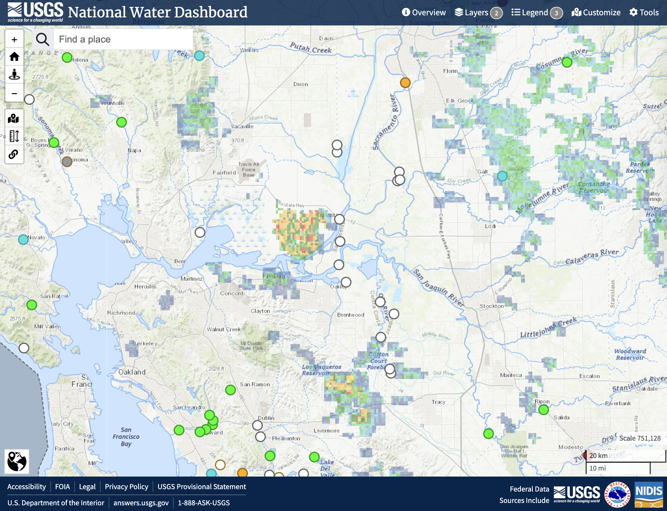
Here is a screenshot of the USGS National Water Dashboard showing monitoring stations (circles) across the Sacramento-San Joaquin Delta in California. Within this region, USGS maintains dozens of monitoring stations that record various parameters over time – often every 15 minutes – with readings archived in many cases for decades.
Many different parameters are available depending on the station and time period. Here are a few examples:
| What is measured | Parameter code | Units |
|---|---|---|
| Discharge (streamflow) | 00060 |
cfs |
| Gage height (water level) | 00065 |
ft |
| Water temperature | 00010 |
°C |
| Specific conductance | 00095 |
μS/cm |
| Turbidity | 63680 |
FNU |
| Dissolved oxygen | 00300 |
mg/L |
| pH | 00400 |
standard units |
4.2 Discover monitoring stations
The read_waterdata_monitoring_location() function is a great starting point for data discovery. It retrieves station metadata and returns an sf spatial data frame that stores station coordinates in a geometry column rather than separate lat/lon columns. Let’s start by searching for all stream gauge stations in California:
# Get all stream gauge stations in California
ca_streams <- read_waterdata_monitoring_location(
  state_name = "California",
  site_type = "Stream"
)
Tip
Note that read_waterdata_monitoring_location() returns an sf spatial object rather than an ordinary data frame. This means coordinates are stored in a geometry column (from the sf package), which spatial filters like st_filter() work, and you can map stations directly with ggplot2 + geom_sf() or leaflet without extra coordinate wrangling.
To narrow results to a smaller region, use sf::st_filter() with a bounding box:
# Build a bounding box for a region of interest, then filter spatially
delta_bbox <- sf::st_bbox(c(xmin = -122.1, ymin = 37.8,
xmax = -121.2, ymax = 38.5),
crs = sf::st_crs(4326))
delta_sites <- sf::st_filter(ca_streams, sf::st_as_sfc(delta_bbox))
# How many stations?
nrow(delta_sites)
# Preview results (geometry column is retained automatically)
delta_sites |>
select(monitoring_location_id, monitoring_location_name) |>
head(10)- 1
- The bounding box covers the core Sacramento-San Joaquin Delta, from roughly Antioch in the west to Stockton in the east and Sacramento in the north.
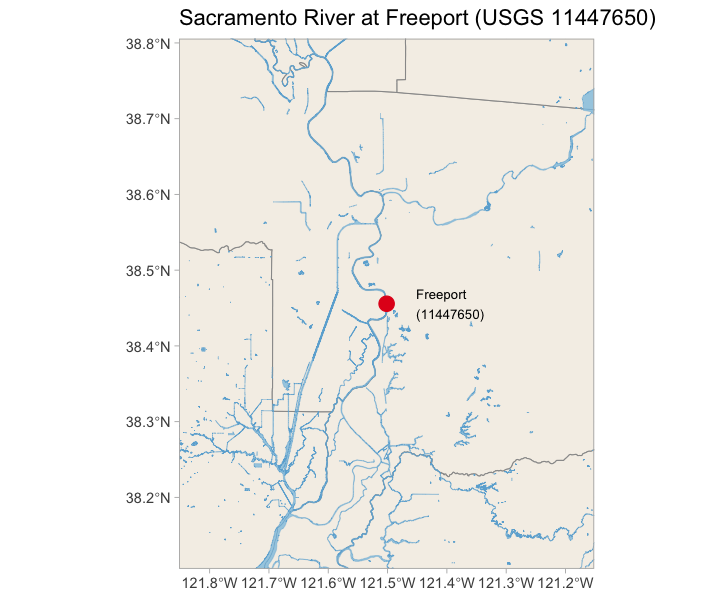
Among the returned stations, you’ll find Sacramento River at Freeport (station USGS-11447650). Freeport sits on the Sacramento River just south of Sacramento, making it a key reference point for water entering the Delta from the north.
TipBonus step: Map the stations
Since delta_sites is an sf object with point geometries, you can visualize the station on a map. Here we use the tigris package to obtain Census TIGER/Line water polygons and county boundaries for the basemap. The counties to fetch are determined automatically from the station’s map extent, with needing to hardcode county names.
options(tigris_use_cache = TRUE)
# Station of interest (already an sf object from delta_sites)
freeport <- delta_sites |>
filter(monitoring_location_id == "USGS-11447650")
# Compute map extent: ±0.35° around the station
lon <- as.numeric(sf::st_coordinates(freeport)[1, "X"])
lat <- as.numeric(sf::st_coordinates(freeport)[1, "Y"])
buf <- 0.35
map_xlim <- c(lon - buf, lon + buf)
map_ylim <- c(lat - buf, lat + buf)
# Find counties intersecting the visual extent
vis_rect <- sf::st_sfc(
sf::st_polygon(list(matrix(c(
map_xlim[1], map_ylim[1], map_xlim[2], map_ylim[1],
map_xlim[2], map_ylim[2], map_xlim[1], map_ylim[2],
map_xlim[1], map_ylim[1]
), ncol = 2, byrow = TRUE))),
crs = sf::st_crs(4326)
)
all_ca <- counties(state = "CA", year = 2022, progress_bar = FALSE)
area_counties <- sf::st_filter(all_ca,
sf::st_transform(vis_rect, sf::st_crs(all_ca)))
# Water-body polygons for those counties
area_water_sf <- map(area_counties$NAME,
~area_water("CA", county = .x, year = 2022)) |>
bind_rows()
# Extract Freeport station coordinates for the text label (avoids
# geom_sf_text CRS warning)
site_coords <- as.data.frame(sf::st_coordinates(freeport))
ggplot() +
geom_sf(data = area_counties, fill = "#f5f0e8",
color = "gray60", linewidth = 0.3) +
geom_sf(data = area_water_sf, fill = "#a6cee3",
color = "#6baed6", linewidth = 0.1) +
geom_sf(data = freeport, color = "#e31a1c",
size = 4, shape = 21, fill = "#e31a1c") +
geom_text(data = site_coords,
aes(x = X, y = Y, label = "Freeport\n(11447650)"),
nudge_x = 0.05, hjust = 0, size = 2.8) +
coord_sf(xlim = map_xlim, ylim = map_ylim, expand = FALSE) +
labs(title = "Sacramento River at Freeport (USGS 11447650)",
x = NULL,
y = NULL) +
theme_light() +
theme(panel.background = element_rect(fill = "#e8f4f8"))- 1
- Caches downloaded TIGER/Line shapefiles locally so repeat runs don’t re-download.
- 2
-
as.numeric()strips the matrix column name so the coordinate works cleanly in arithmetic.
NoteWhat is
tigris?
The tigris package downloads US Census Bureau TIGER/Line shapefiles directly into R as sf objects. These contain the same boundaries and geographic features used for the US Census, updated every few years.
For station maps, two functions are especially useful:
counties(state, year): county boundaries for any US statearea_water(state, county, year): areal water bodies: rivers (as polygons), lakes, bays, and estuaries.
Setting options(tigris_use_cache = TRUE) tells tigris to save downloaded shapefiles to a local cache folder. Repeat calls load from disk instantly with no network request.
4.3 Explore data availability
Before downloading, it’s worth checking what’s actually available at a station. read_waterdata_combined_meta() returns a row for each monitored parameter at a site:
# What data does Freeport have?
freeport_avail <- read_waterdata_combined_meta(
  monitoring_location_id = "USGS-11447650"
)

# Which parameters are available, and for how long?
freeport_avail |>
  select(parameter_code, parameter_name, statistic_id, begin, end) |>
  arrange(parameter_code, statistic_id)
Look for your desired parameter(s) in the results. The begin and end timestamps show the period of record. It’s useful to consult this information before constructing your data retrieval code, because there’s no point requesting data outside that range!
Notice that water temperature (00010) appears multiple times, with different statistic_id values. This is because the API stores separate time series for each computed statistic:
freeport_avail |>
  filter(parameter_code == "00010") |>
  count(statistic_id)
Although you can manually look up names and descriptions of all possible statistic codes in a browser, you can also retrieve this information directly via the package:
stat_codes <- read_waterdata_metadata("statistic-codes")

# Show statistic names along with other station availability data
freeport_avail %>%
  filter(parameter_code == "00010") %>%
  select(parameter_code, parameter_name, statistic_id, begin, end) %>%
  left_join(stat_codes, by = join_by(statistic_id == statistic_code)) %>%
  select(-statistic_description) %>%
  relocate(statistic_name, .after = statistic_id) %>%
  arrange(parameter_code, statistic_id)
The four codes you’ll typically see for daily temperature are daily maximum (00001), daily minimum (00002), daily mean (00003), and instantaneous values (00011). When you call read_waterdata_daily(), you select which statistic you want by passing statistic_id.
4.4 Retrieve daily water temperature data
read_waterdata_daily() retrieves daily values. We pass parameter_code = "00010" to select water temperature and statistic_id = "00003" to select the daily mean, and wrap the call in our caching pattern:
freeport_temp_file <- "data/freeport_temp.rds"
if (!file.exists(freeport_temp_file)) {
message("Fetching daily temperature from USGS...")
freeport_temp <- read_waterdata_daily(
monitoring_location_id = "USGS-11447650", # note "USGS-" prefix
parameter_code = "00010", # water temperature
statistic_id = "00003", # daily mean
time = c("2020-01-01", "2023-12-31")
)
dir.create("data", showWarnings = FALSE)
saveRDS(freeport_temp, freeport_temp_file)
} else {
freeport_temp <- readRDS(freeport_temp_file)
}
glimpse(freeport_temp)- 1
-
The new API requires the
"USGS-"prefix on all site numbers. Old functions accepted bare numbers like"11447650".
The returned data is in long format, with one row per observation. Note that the result is an sf object – it retains the station’s geometry column – so you can join or map it directly without extra steps.
TipUnderstanding approval status
The approval_status column tells you whether a value has been reviewed. "Approved" means a USGS hydrologist has checked and signed off on the data. "Provisional" means the data is real-time and hasn’t been reviewed yet. For analyses using historical data, filter to approval_status == "Approved" if data quality is critical.
4.5 Visualize the data
A time series plot is the natural first look at the data:
ggplot(freeport_temp, aes(x = time, y = value)) +
  geom_line(color = "#e34a33", alpha = 0.6, linewidth = 0.3) +
  labs(
    x = NULL,
    y = "Temperature (°C)",
    title = "Daily Mean Water Temperature at the Sacramento River near Freeport",
    subtitle = "USGS Station 11447650 (2020-2023)"
  ) +
  theme_light()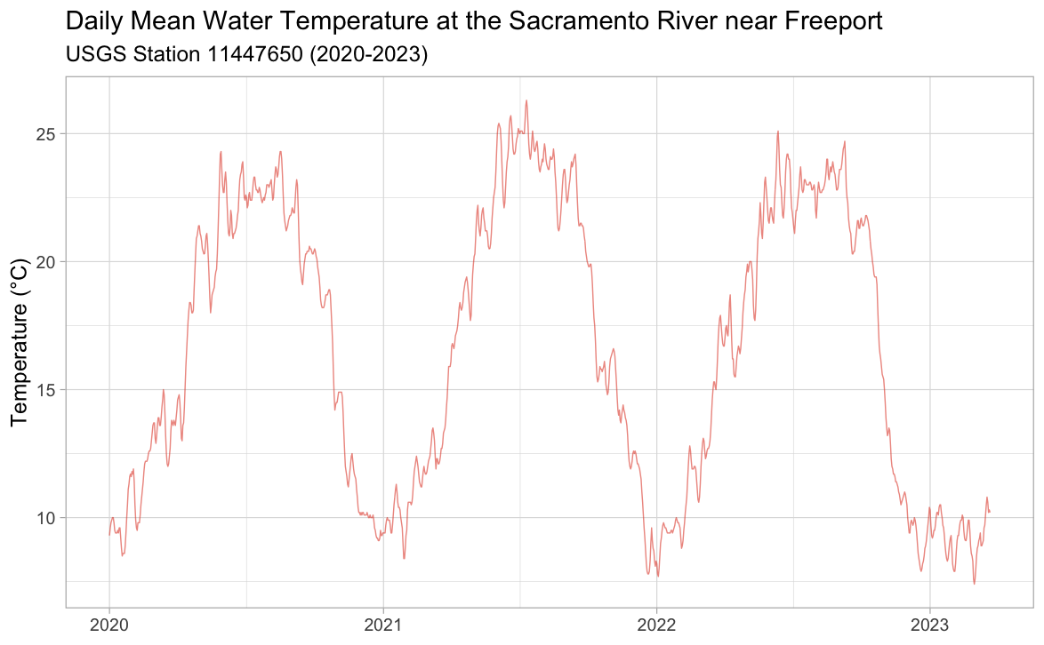
4.5.1 Seasonal patterns
A monthly boxplot makes the seasonal structure explicit:
freeport_temp |>
  mutate(month = month(time, label = TRUE)) |>
  ggplot(aes(x = month, y = value)) +
  geom_boxplot(fill = "#8abcfd", outlier.alpha = 0.2, outlier.size = 0.5) +
  labs(
    x = "Month",
    y = "Temperature (°C)",
    title = "Seasonal Temperature Distribution",
    subtitle = "Sacramento River near Freeport (2020-2023)"
  ) +
  theme_light()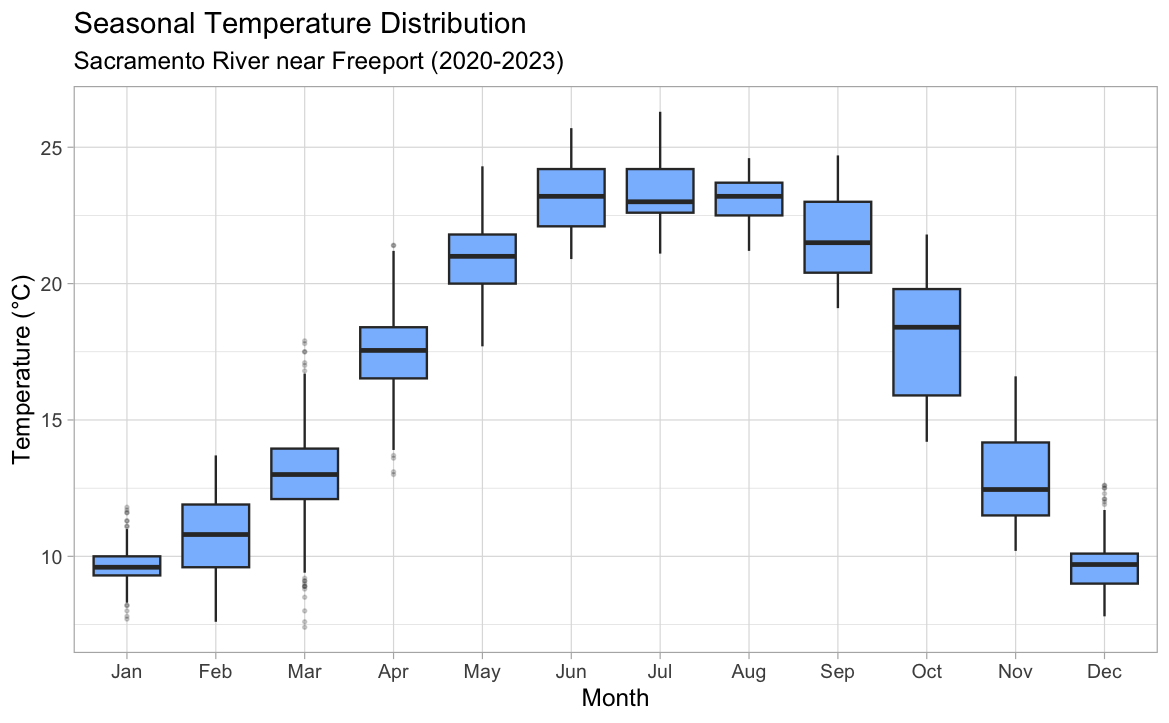
4.6 Retrieving additional parameters
The same workflow retrieves any other parameter at Freeport. For example, here’s a very similar function call for getting daily mean suspended sediment concentration:
freeport_ss <- read_waterdata_daily(
  monitoring_location_id = "USGS-11447650",
  parameter_code = "80154",  # suspnd sedmnt conc
  statistic_id = "00003",  # daily mean
  time = c("2020-01-01", "2023-12-31")
)
# value column holds the daily mean suspended sediment concentration in mg/L
TipFetching multiple parameters in one call
Pass a vector of parameter codes to retrieve several parameters at once. The result is still long format (i.e., one row per observation) with parameter_code identifying which parameter each row belongs to:
multi <- read_waterdata_daily(
  monitoring_location_id = "USGS-11447650",
  parameter_code = c("00010", "00060", "80154"),  # temp, discharge, susp sedmnt conc
  statistic_id = "00003",  # daily mean for all three
  time = c("2020-01-01", "2023-12-31")
)

# Plot time series faceted by parameter
multi %>%
  ggplot(aes(x = time, y = value, col = parameter_code)) +
  geom_line() +
  facet_wrap(~parameter_code, scales = "free_y", ncol = 1)
One call, three parameters, all stacked in long format, easy to filter or facet!
TipWater Quality Portal: beyond USGS
dataRetrieval also connects to the Water Quality Portal, which aggregates data from USGS, EPA, and over 400 state and local agencies. Use readWQPdata() to query this broader dataset:
# Water quality data from all agencies at a USGS site
wq <- readWQPdata(
  siteid = "USGS-11447650",
  characteristicName = "Turbidity"
)
This is particularly useful for parameters like nutrients, metals, or biological data that NWIS doesn’t collect but state environmental agencies often do.
5 Under the Hood: How APIs Work
We just retrieved many months of streamflow data with a handful of function calls. But what was actually happening? Understanding the mechanics will help you work with any API, including ones that don’t have a ready-made R package.
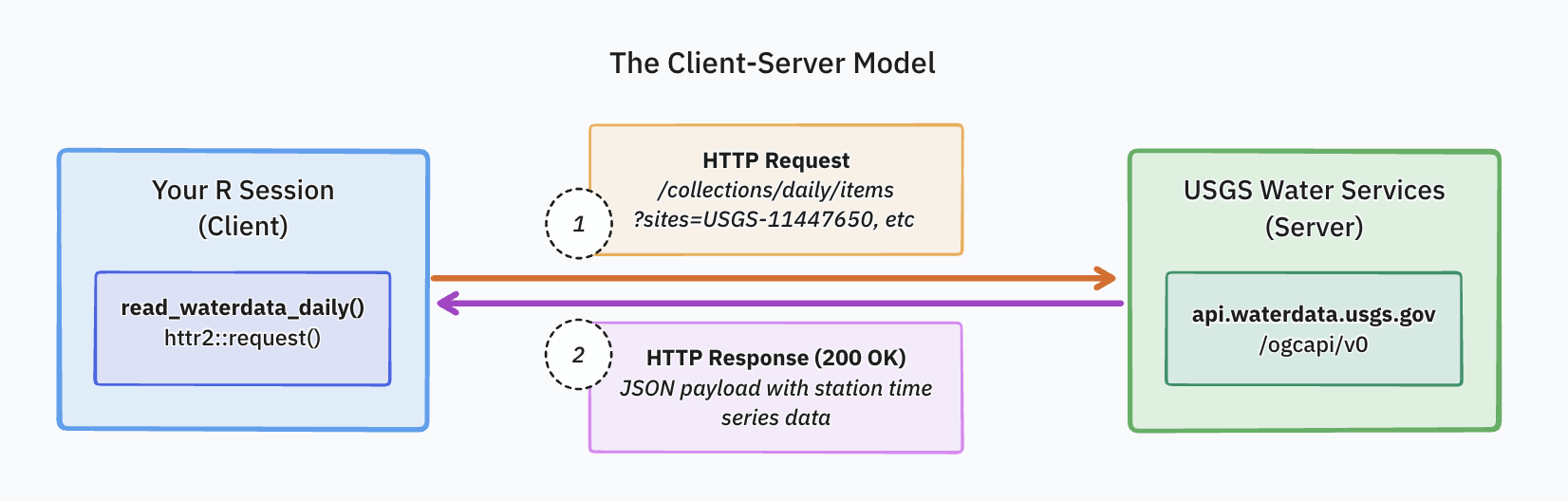
5.1 The client-server model
When you call read_waterdata_daily(), your R session (the client) sends a structured request across the internet to the USGS water services server. The server uses information in the request to perform some action(s) – e.g., query its database for the requested data – and then sends a response back.
5.2 Anatomy of an API request
Every request to a web API is ultimately a URL. Here’s what read_waterdata_daily(monitoring_location_id = "USGS-11447650", parameter_code = "00010", statistic_id = "00003", time = c("2020-01-01", "2020-01-05")) constructs behind the scenes:
https://api.waterdata.usgs.gov/ogcapi/v0/collections/daily/items?f=json&lang=en-US&monitoring_location_id=USGS-11447650¶meter_code=00010&statistic_id=00003&time=2020-01-01%2F2020-01-05&limit=50000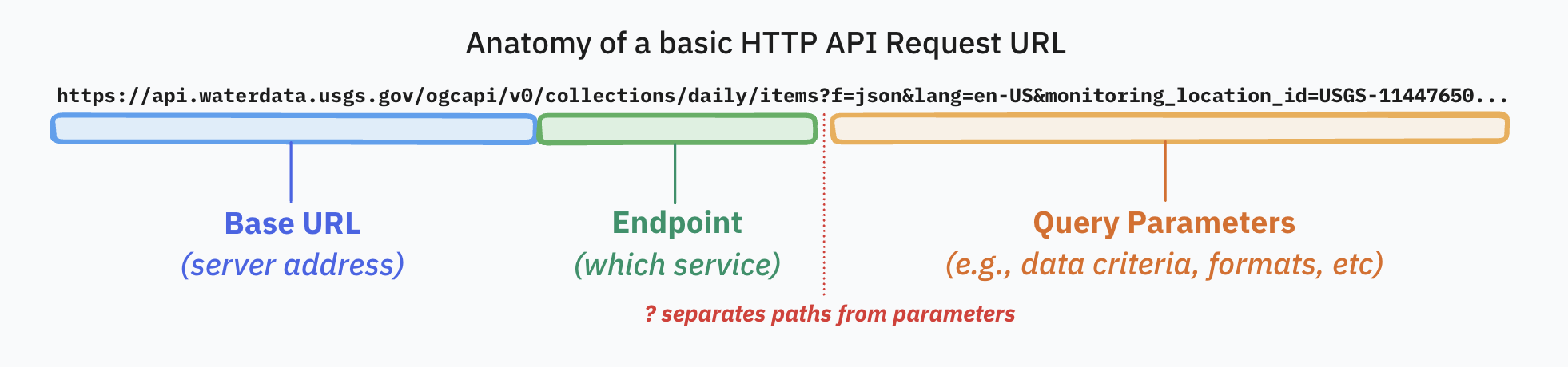
Try it yourself: paste that URL into a browser. The raw JSON data that dataRetrieval processes for you will appear as text in the browser window.
5.3 What the server sends back
An HTTP response has two key parts:
- A status code: a number indicating success or failure.
200– success404– resource not found429– too many requests (you’re being rate-limited)500– server error
- A response body: the actual data, typically as JSON, CSV, or XML.
dataRetrieval handles all of this automatically. It builds the URL, sends the request, checks the status, and parses the JSON body into a tidy R data frame. Most of the time, that’s exactly what you want. When no R package exists for an API you need, httr2 lets you do these steps yourself.
6 Optional: Building Custom API Requests with httr2
NoteThis section is optional
Skip ahead to Your Turn if time is short. The techniques here are useful when you need to work with an API that has no dedicated R package, but you won’t need them otherwise.
The httr2 package provides a pipe-based interface for building and sending HTTP requests. Think of it as doing manually what dataRetrieval does automatically.
NoteSetup
install.packages("httr2")
library(httr2)
6.1 The httr2 workflow
httr2 separates building a request from executing it. You assemble everything first, then send it:
# Build the same request that read_waterdata_daily() constructs
req <- request("https://api.waterdata.usgs.gov/ogcapi/v0") |>
req_url_path_append("/collections/daily/items") |>
req_url_query(
monitoring_location_id = "USGS-11447650",
parameter_code = "00010",
statistic_id = "00003",
time = "2020-01-01/2020-01-05" # ISO 8601 interval format
)
# Preview the request without actually sending it
req_dry_run(req)- 1
-
req_dry_run()prints the exact URL and headers that would be sent.
Once you’re happy with the request structure, execute it:
# Send the request, returning a response
resp <- req_perform(req)

# Check the HTTP status code
resp_status(resp)  # 200 = success

# Parse the JSON response body
resp_body_json(resp)6.3 When to use httr2 vs. a package
| Situation | Use |
|---|---|
A well-maintained R package exists (dataRetrieval, rgbif, dataone, …) |
The package |
| An API exists but no R package wraps it | httr2 |
| You need request features the package doesn’t expose | httr2 |
| You’re building your own R package around an API | httr2 as the foundation |
7 Your Turn
NoteActivity: Retrieve and visualize water data
Working individually or in pairs (10 min), choose one of the following:
Option A: Different station: Retrieve daily mean water temperature (parameter_code = "00010", statistic_id = "00003") for one of these other nearby stations and compare the seasonal pattern with Freeport. Is the annual cycle the same shape? Earlier or later in the year?
- San Joaquin River at Vernalis:
USGS-11303500 - Cache Slough near Ryer Island:
USGS-11455385 - Sacramento River at Rio Vista:
USGS-11455420
Option B: Different statistic: At Freeport (USGS-11447650), retrieve the daily maximum (statistic_id = "00001") and daily minimum ("00002") temperature in addition to the mean. Plot all three on one time series. How wide is the daily range? Does it vary by season?
Option C: Temperature vs. discharge: Retrieve both daily mean temperature (00010) and daily mean suspended sediment concentration (80154) at Freeport. Make a scatter plot. Is there a clear relationship? What might you look at next?
Include the cache pattern in your code so it only downloads once!
8 Resources
- dataRetrieval package documentation – function reference, vignettes, and worked examples
- USGS National Water Dashboard – interactive map for exploring monitoring stations before querying with R
- USGS NWIS Parameter Codes – look up parameter codes and descriptions (or use
dataRetrieval::parameterCdFilein R) - Water Quality Portal – access water quality data from USGS, EPA, and partner state/local agencies
- USGS NWIS Web Services – documentation for the REST API that
dataRetrievaluses under the hood - httr2 documentation – full reference for building custom API requests in R