Writing Functions – 2026 Delta Synthesis Working Groups week 2 (April 2026)

Learning Objectives

After completing this session, you will be able to:

Explain the importance of using and developing functions
Create custom functions using R code
Document functions to improve understanding and code communication

1 Setup

### For data wrangling and plotting
library(dplyr)
library(tidyr)
library(ggplot2)
library(purrr) ### for iteration using map() family of functions

library(palmerpenguins) ### example data

2 Why Functions?

Many R users write code as a continuous stream of commands—paste from the console, run, repeat. That works, but breaking code into small, reusable functions pays off quickly.

The guiding principle is DRY: Don’t Repeat Yourself. If you’ve copied and pasted a block of code more than twice, it’s time to write a function. Functions give you:

Less repetition — change logic in one piece of code, not ten
Fewer errors — one tested implementation instead of many copies
Better readability — a well-named function documents the coder’s intent

2.1 Function Basics

The syntax for defining a function in R is:

my_function <- function(argument1, argument2) {
  <code that performs some well defined task>
  return(result)
}

You can call it just like any built-in function:

result <- my_function(argument1 = value1, argument2 = value2)

Naming Functions

Ideally, function names should be short, but still clearly capture what the function does.

Best Practices from Chapter 19 Functions in R for Data Science:

Function names should be verbs and arguments should be nouns (there are exceptions).
Use the snake_case naming convention for functions that are multiple words.
For a “family” of functions, use a common prefix to indicate that they are connected. For example, most of the functions in the usethis package have the prefix use_*

Based on these tips, is my_function() a good name for a function?

2.2 Example: Temperature Conversion

Imagine you have some temperature data measured in degrees Fahrenheit and you want to convert that to Celsius for your analysis. You might have an R script that does this for you.

airtemps <- c(212, 30.3, 78, 32)
celsius1 <- (airtemps[1] - 32) * 5/9
celsius2 <- (airtemps[2] - 32) * 5/9
celsius3 <- (airtemps[3] - 33) * 5/9

Here we repeat the same formula three times. And note the third time, there’s a subtle mistake! This code would be both more compact and more reliable if we didn’t repeat ourselves.

Convert Fahrenheit to Celsius

To create a function in R, we use the function function (so meta!) and assign its result to an object. Let’s create a function that calculates Celsius temperature outputs from Fahrenheit temperature inputs.

convert_f_to_c <- function(fahr) {
  celsius <- (fahr - 32) * 5/9
  return(celsius)
}

Because R operations are vectorized, this works on a single value or an entire vector:

### check single value:
celsius1a <- convert_f_to_c(airtemps[1])
celsius1a == celsius1

[1] TRUE

### calculate for whole vector:
celsius_vec <- convert_f_to_c(airtemps)
celsius_vec

[1] 100.0000000  -0.9444444  25.5555556   0.0000000

Exercise - Convert Celsius to Fahrenheit

Write a function convert_c_to_f that reverses the conversion. Use it to convert celsius back to Fahrenheit and verify that the result matches airtemps.

Hint: the formula for Celsius to Fahrenheit conversions is celsius * 9/5 + 32.

Answer

convert_c_to_f <- function(celsius) {
    fahr <- celsius * 9/5 + 32
    return(fahr)
}

fahr_vec <- convert_c_to_f(celsius_vec)
airtemps == fahr_vec

[1] TRUE TRUE TRUE TRUE

3 Functions: Input, Output, Environment

3.1 Setting Argument Defaults

Function arguments often include a default value - in which case, the user can opt to simply not assign a value. Here, convert_temp() allows the user to specify the scale of their input, defaulting to Fahrenheit (scale = 'f').

convert_temp <- function(t, scale = 'f') {
    if(scale == "c") {
        result = t * 9/5 + 32
    } else {
        result  = (t - 32) * 5/9
    }
    return(round(result, 3))
}

convert_temp(t = airtemps)

[1] 100.000  -0.944  25.556   0.000

convert_temp(t = airtemps, scale = 'Celsius')

[1] 100.000  -0.944  25.556   0.000

3.2 Error handling!

Sometimes a user will include an argument that breaks the code - a character when the function expects a number, upper-case when expecting lower-case, etc. Try to anticipate simple errors and include a way to identify and handle them in the function: try to correct the error on the fly, or use stop() to return a useful error message to the user.

Consider some common mistakes a usermight make with convert_temp() and how might we deal with them?

convert_temp <- function(t, scale = 'f') {
    scale = tolower(substr(scale, 1, 1))
    if(!scale %in% c('c', 'f')) {
      stop('scale must be either "c" or "f"')
    }
    if(scale == "c") {
        result = t * 9/5 + 32
    } else {
        result  = (t - 32) * 5/9
    }
    return(round(result, 3))
}

1: What if user enters scale = "Celsius"? substr(x, 1, 1) grabs just the first letter, and tolower forces it to lower case
2: If scale is not one of the expected values, generate a sensible error with stop()
3: We know the values are valid now, so we can use a simple if/else to do the correct calculation!

3.3 Returning Values

Use return(x) to end the function and hand the resulting value back to the user. To provide multiple values back to a user, consider more complex data structures like a dataframe (well structured) or a named list (very flexible).

convert_f_to_c_k <- function(f) {
  c <- (f - 32) * 5/9
  k  <- c + 273.15
  out_df <- data.frame(fahr = f, celsius = c, kelvin = k)
  return(out_df)
}

temps_df <- convert_f_to_c_k(seq(-100, 100, 50))
temps_df

  fahr   celsius   kelvin
1 -100 -73.33333 199.8167
2  -50 -45.55556 227.5944
3    0 -17.77778 255.3722
4   50  10.00000 283.1500
5  100  37.77778 310.9278

convert_f_to_c_k <- function(f) {
  c <- (f - 32) * 5/9
  k  <- c + 273.15
  out_list <- list(fahr = f, celsius = c, kelvin = k)
  return(out_list)
}

temps_list <- convert_f_to_c_k(seq(-100, 100, 50))
temps_list

$fahr
[1] -100  -50    0   50  100

$celsius
[1] -73.33333 -45.55556 -17.77778  10.00000  37.77778

$kelvin
[1] 199.8167 227.5944 255.3722 283.1500 310.9278

Without an explicit return() we might get unexpected results!

convert_f_to_c_k <- function(f) {
  c <- (f - 32) * 5/9
  k  <- c + 273.15
  out_list <- list(fahr = f, celsius = c, kelvin = k)
  print('calculation successful!')
}

temps_oops <- convert_f_to_c_k(seq(-100, 100, 50))

[1] "calculation successful!"

temps_oops

[1] "calculation successful!"

Implicit vs explicit return()

If you don’t explicitly state a value to return(), R will pass the result of the last step of the function. For simple functions, this is fine, but for anything more than a line or two, best practice is to explicitly call return() so it is obvious what is being returned.

3.4 Functions and Environments

When a function is called, it exists in some environment within R; this is its parent environment (when working interactively this is the global environment). The function performs all its calculations in a temporary environment, child of the parent. When the function completes, it returns a value to the parent then that temporary child environment disappears, taking any intermediate values with it. This can cause confusing behavior.

a <- 1       ### create object a in parent environment

add_one <- function(x) {
  x <- x + 1 ### increment argument by 1
  a <- a + 2 ### modify a in function environment
  b <- a + 3 ### create b in function environment
  return(x)  ### only x is returned back to parent
}

add_one(a)   ### give `a` as arg to the function; returns the value a + 1

[1] 2

a            ### value in parent env is unchanged by calcs in the function

[1] 1

exists('b')  ### objects created in the function disappear when function ends

[1] FALSE

In the above example, there is no starting value of a in the child (function) environment, but like a good parent-child relationship, the child can look “up” to the parent if it can’t find a needed value (a in parent environment) within its own environment. However, the change in a (and the creation of b) within the child environment are lost when the function ends - like a bad parent-child relationship, the child is abandoned and forgotten!

There are complexities and ways to get around this behavior, but it’s best just to be aware, and make sure any values the user needs get sent back to the parent environment using return()!

4 Functions: Use Cases

Functions are amazing for reusing common code logic and for communicating the intent of a block of code by assigning a name. But functions can make it much easier to iterate complex operations on vectors and lists, and can help you create customized plot themes that you can use across multiple plots to maintain a consistent “brand”.

4.1 Functions for Iteration

A function allows you to easily reuse a piece of code. This is especially powerful when coupled with iteration functions: *apply functions (base R) and the map_* functions from the purrr package. For example, you could apply a function to each element of a list or vector in sequence; separate a dataframe into pieces by some variable, then fit a model to each piece or generate a separate plot for each; or read in a series of separate data files and summarize the results into a complete dataframe.

The apply and map functions typically take a list or vector for their first argument, and a function as their second.

The first argument of the function .x or X should generally be the variable being iterated over!
The function argument .f or FUN should not have parentheses after it!

Apply the square root function sqrt() to each element of a vector of numbers. NOTE, if nums were a vector, this would be trivial since sqrt already takes advantage of vectorization; here we made nums a list just for fun.

nums <- list(1, 3, 9, 49, 101, pi)
purrr::map_vec(.x = nums, .f = sqrt)
base::sapply(X = nums, FUN = sqrt)

1: map() always returns a list, but map_vec simplifies into a vector; see also map_df or type-specific versions like map_int, map_chr, or map_dbl
2: apply() returns various formats depending on output; sapply returns the results simplified into a vector or matrix

[1]  1.000000  1.732051  3.000000  7.000000 10.049876  1.772454
[1]  1.000000  1.732051  3.000000  7.000000 10.049876  1.772454

Let’s take the palmerpenguins::penguins dataset and create a linear model of bill length vs bill depth for each of the three penguin species, Chinstrap, Adelie, and Gentoo. Note, there are more efficient ways to do this, here we are spelling it out as a teaching case.

library(palmerpenguins)
data(penguins)
spp_vec <- unique(penguins$species)

calc_bill_model <- function(spp, df) {
    spp_df <- df %>%
        filter(species == spp)
    bill_mdl <- lm(bill_length_mm ~ bill_depth_mm, data = spp_df)
    return(bill_mdl)
}
map_results <- purrr::map(.x = spp_vec, .f = calc_bill_model, df = penguins)
broom::tidy(map_results[[3]])
lapply_results <- base::lapply(X = spp_vec, FUN = calc_bill_model, df = penguins)
broom::tidy(lapply_results[[3]])

1: map() always returns a list, which works well for storing a complex object like a linear model
2: broom::tidy() summarizes a model object into a nice clean dataframe
3: lapply() always returns a list, which works well for storing a complex object like a linear model

# A tibble: 2 × 5
  term          estimate std.error statistic       p.value
  <chr>            <dbl>     <dbl>     <dbl>         <dbl>
1 (Intercept)      13.4      5.06       2.66 0.00992      
2 bill_depth_mm     1.92     0.274      7.01 0.00000000153
# A tibble: 2 × 5
  term          estimate std.error statistic       p.value
  <chr>            <dbl>     <dbl>     <dbl>         <dbl>
1 (Intercept)      13.4      5.06       2.66 0.00992      
2 bill_depth_mm     1.92     0.274      7.01 0.00000000153

Named Functions vs Anonymous Functions

In the examples above, we used named functions (sqrt defined in base R, calc_bill_model defined by our own code). The map and apply functions also work well with anonymous functions - small tasks where the code is only needed once and can be discarded after. The function is created on the fly and not assigned to a named object.

Using function() but not assigning it to an object, just giving it directly to the FUN argument.

base::sapply(X = 1:3, FUN = function(x) x + 1)

[1] 2 3 4

R 4.1 introduced a shorthand for function(args) {expr} using a backslash: \(args) expr:

base::sapply(X = 1:3, FUN = \(x) x + 1)

[1] 2 3 4

The purrr package uses a tilde-dot syntax as placeholder for the argument. It also works with function() or the backslash shorthand.

purrr::map_vec(.x = 1:3, .f = ~ .x + 1)

[1] 2 3 4

purrr::map_vec(.x = 1:3, .f = \(x) x + 1)

[1] 2 3 4

4.2 Functions for Custom Plot Themes

If you make many similar plots, a custom theme function keeps formatting consistent and easy to update (we know this is not the greatest plot, we’re just changing various aspects that should be obvious in the resulting plot).

custom_theme <- function(base_size = 9) {
  theme(
    text             = element_text(family = "serif",
                                    color  = "slateblue4",
                                    size   = base_size),
    plot.title       = element_text(size   = rel(1.25),
                                    hjust  = 0.5,
                                    face   = "bold"),
    panel.background = element_rect(color = 'slateblue3',
                                    fill  = 'azure'),
    panel.grid.major = element_line(color    = "slateblue1",
                                    linewidth = 0.25),
    legend.position  = c(.9, .4),
    axis.ticks       = element_line(color = 'red')
  )
}

You can go further and wrap the entire plot in a function too:

scatterplot <- function(df, point_size = 2, font_size = 9) {
  ggplot(data = df, mapping = aes(x = fahr, y = celsius, color = kelvin)) +
    geom_point(size = point_size) +
    scale_color_viridis_c() +
    custom_theme(font_size)
}

scatterplot(temps_df, point_size = 3, font_size = 16) +
  labs(title = 'Temperature Conversions')

1: Since scatterplot() returns a ggplot object, we can continue to add ggplot layers - additional geoms, scales, labels, etc.

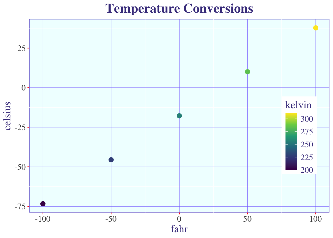
Now all plots built with scatterplot() can be reformatted by changing one function – whether you’re making 1, 10, or 100 plots.

5 Documenting Functions

Well-named functions are a start, but good documentation tells collaborators (and future you) what a function expects and what it returns. Comments in the function body are a good start. For a more standardized structure, the roxygen2 package provides a lightweight format for this. Place comments starting with #' immediately above the function definition, and use specific tags (e.g., @param) to define sections of the documentation.

#' Convert temperature from Fahrenheit to Celsius
#'
#' @param fahr Numeric value or vector in degrees Fahrenheit
#'
#' @returns Numeric value or vector in degrees Celsius
#' @export
#'
#' @examples
#' convert_f_to_c(32)
#' convert_f_to_c(c(32, 212, 72))
convert_f_to_c <- function(fahr) {
  celsius <- (fahr - 32) * 5/9
  return(celsius)
}

Key tags:

Tag	Purpose
`@param`	Describes each input argument to the function
`@returns`	Describes the function’s output
`@examples`	Shows usage examples
`@export`	Makes the function available if bundled in a package

This roxygen2 structure might seem overly complicated, but it will be useful for others interested in using your functions (including “future you”) - especially when including your functions in an R package!

Note

For more best practices on function documentation, check out Hadley Wickham and Jennifer Bryan’s online book R Packages (2e) - Chapter 10, Section 16: Function Documentation.

6 Exercises

In this sequence of exercises, we will build up a function to calculate the weight of Chinook salmon based only on length, using a simple length-to-width formula \(W = aL^b\).

Exercise - Create basic model

Write a function that takes salmon length, in inches, and returns the corresponding weight, in pounds. The simple model is \(W = aL^b\); for Chinook salmon, let’s use \(a=0.00057\) and \(b=2.9\) (for inches to pounds). Give it a name that indicates the purpose of the function. For testing purposes, a 30” salmon should be about 11 lb; a 42” salmon is about 27 lb; and a 60” is about 82 lb.

Answer

fish_l_to_w <- function(L) {
    a <- .00057
    b <- 2.9
    W <- a * L^b
    return(round(W, 2))
}
test_vec <- c(30, 42, 60)
fish_l_to_w(L = test_vec)

[1] 10.95 29.06 81.75

Exercise - Generalize with default arguments

The formula \(W = aL^b\) is useful for many different fish species, but the \(a\) and \(b\) values differ from species to species. Generalize the function in two ways:

Allow the user to provide different values for \(a\) and \(b\), but use the values for salmon as the default.
Allow the user to provide length in inches or centimeters, with an argument so the user can specify “in” or “cm”.

To test the functionality, a California kelp bass model might use \(a=0.000779\) (for length in inches) and \(b=3.01\); a 12-inch bass is about 1.4 lb, while a 22 inch is about 8.5 lb.

Answer

fish_l_to_w <- function(L, a = 0.00057, b = 2.9, units = "in") {
    if(units == "cm") {
      length_in <- L / 2.54
    } else length_in <- L
    W <- a * length_in^b           ### use length_in instead of L
    if(units == "cm") W <- W / 2.2 ### convert lb to kg to keep in metric
    return(round(W, 2))
}
test_vec <- c(30, 42, 60)
fish_l_to_w(L = test_vec)

[1] 10.95 29.06 81.75

fish_l_to_w(L = test_vec * 2.54, units = "cm")

[1]  4.98 13.21 37.16

### test kelp bass
fish_l_to_w(L = c(12, 22), a = 0.000779, b = 3.01)

[1] 1.38 8.56

Exercise - Add error handling

What kinds of errors might someone make when applying this function - either misunderstandings or typos? Some things we might check:

\(a\) should be a number between 0 and 1 (usually very small); \(b\) should be greater than 1 (usually close to 3, since volume ~ cube of linear dimensions).
A user might type the full unit name, or units that aren’t supported.
What other errors might a user make?

Answer

fish_l_to_w <- function(L, a = 0.00057, b = 2.9, units = "in") {
    if(!is.numeric(c(a, b))) stop('Both `a` and `b` must be numeric!')
    if(a < 0 | a > 1) stop('The `a` parameter should be between 0 and 1!')
    if(b < 1) stop('The `b` parameter should be greater than 1!')
    if(!tolower(units) %in% c('in', 'cm')) stop('The units should be either `in` or `cm`!')
    
    if(units == "cm") {
      length_in <- L / 2.54
    } else length_in <- L
    W <- a * length_in^b           ### use length_in instead of L
    if(units == "cm") W <- W / 2.2 ### convert lb to kg to keep in metric
    return(round(W, 2))
}

fish_l_to_w(L = 30, a = -.0003)

[1] "The `a` parameter should be between 0 and 1!"

Exercise - Add documentation

Create some basic documentation for your function using the roxygen2 syntax.

Answer

Documentation might look something like this:

#' Fish length-to-width conversion
#' 
#' Convert length of fish to estimated weight using the formula W = aL^b
#' 
#' @param L Fish length in inches or cm
#' @param a The `a` value for the formula *based on L in inches*; default 
#'          0.00057 for Chinook salmon length
#' @param b The `b` value for the formula; default 2.9 for Chinook salmon
#' @param units The units of the given length, in inches (default) or cm.
#' 
#' @returns Numeric value or vector of fish weight in lb (if units = "in") or 
#'          mass in kg (if units = "cm")
#' 
#' @export
#' 
#' @examples
#' fish_l_to_w(L = c(24, 60))

fish_l_to_w <- function(L, a = 0.00057, b = 2.9, units = "in") {
    if(a < 0 | a > 1) stop('The `a` parameter should be between 0 and 1!')
    if(b < 1) stop('The `b` parameter should be greater than 1!')
    if(!tolower(units) %in% c('in', 'cm')) stop('The units should be either `in` or `cm`!')
    
    if(units == "cm") {
      length_in <- L / 2.54
    } else length_in <- L
    W <- a * length_in^b           ### use length_in instead of L
    if(units == "cm") W <- W / 2.2 ### convert lb to kg to keep in metric
    return(round(W, 2))
}

6.1 Challenge Exercise

Exercise

Use your function to iterate over a list of several species of fish. Copy this code to create a list of fish lengths and parameters:

fish_list <- list(
    chinook_salmon = list(length = c(30, 42, 60), 
                          a = 0.00057, b = 2.9, units = "in"),
    kelp_bass      = list(length = c(12, 22), 
                          a = 0.000779, b = 3.01, units = "in"),
    rainbow_trout  = list(length = c(20, 35, 50), 
                          a = 0.000605, b = 2.87, units = "cm")
)

Hint: you may want to create an anonymous function that takes a list of parameters and feeds them into your fish_l_to_w() function, then use map() or lapply() to apply it to each element of the list.

Answer

purrr::map(.x = fish_list, 
           .f = ~ fish_l_to_w(L = .x$length, 
                              a = .x$a, 
                              b = .x$b, 
                              units = .x$units))

$chinook_salmon
[1] 10.95 29.06 81.75

$kelp_bass
[1] 1.38 8.56

$rainbow_trout
[1] 0.10 0.51 1.42

lapply(X = fish_list, 
       FUN = function(x) fish_l_to_w(L = x$length, 
                                     a = x$a,
                                     b = x$b,
                                     units = x$units))

$chinook_salmon
[1] 10.95 29.06 81.75

$kelp_bass
[1] 1.38 8.56

$rainbow_trout
[1] 0.10 0.51 1.42