### Data wrangling packages:
library(readr)
library(dplyr)
library(tidyr)
library(here)
### Simple Features vector spatial data:
library(sf)
### Data visualization packages:
library(ggplot2)
library(leaflet)
library(ggspatial)
library(prettymapr) ### ggspatial depends on but does not import prettymapr for internal functions1 Scope: Vector, Not Raster
This lesson focuses on working with vector spatial data in R, primarily using the sf “simple features” package in R. Vector spatial data includes spatial points, lines, polygons, and multi-polygon features, each feature described with attributes such as a place name, an ID, or the population associated with the feature.
This lesson does not focus on working with raster spatial data. Raster data is typically a grid of pixels with each pixel containing some value, like elevation or temperature. Satellite imagery and remote sensing data are common examples of raster data.
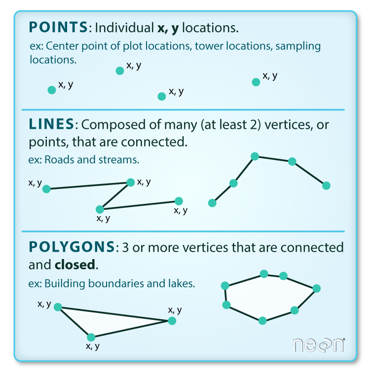
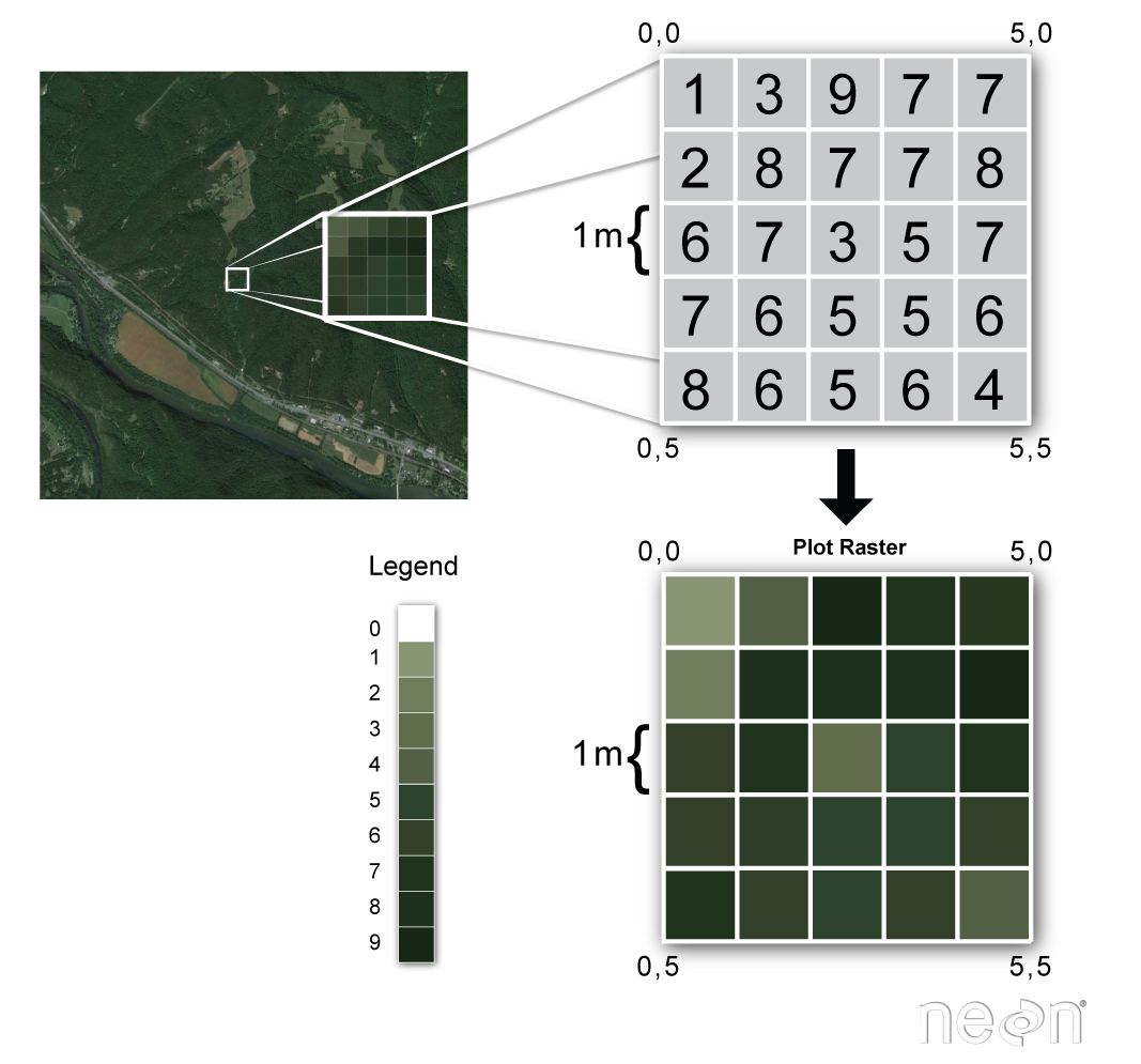
Mastering spatial data in R (or any GIS system) requires a solid understanding of both vector and raster spatial data; at the end of the lesson are some resources to build you up on vector data and get you started with rasters.
2 Brief Introduction to sf
From the sf vignette:
Simple features or simple feature access refers to a formal standard (ISO 19125-1:2004) that describes how objects in the real world can be represented in computers, with emphasis on the spatial geometry of these objects. It also describes how such objects can be stored in and retrieved from databases, and which geometrical operations should be defined for them.
The sf package is an R implementation of Simple Features. This package incorporates:
- a new spatial data class system in R
- functions for reading and writing spatial data
- tools for spatial operations on vectors
Most of the functions in this package starts with prefix st_ which stands for spatial and temporal.
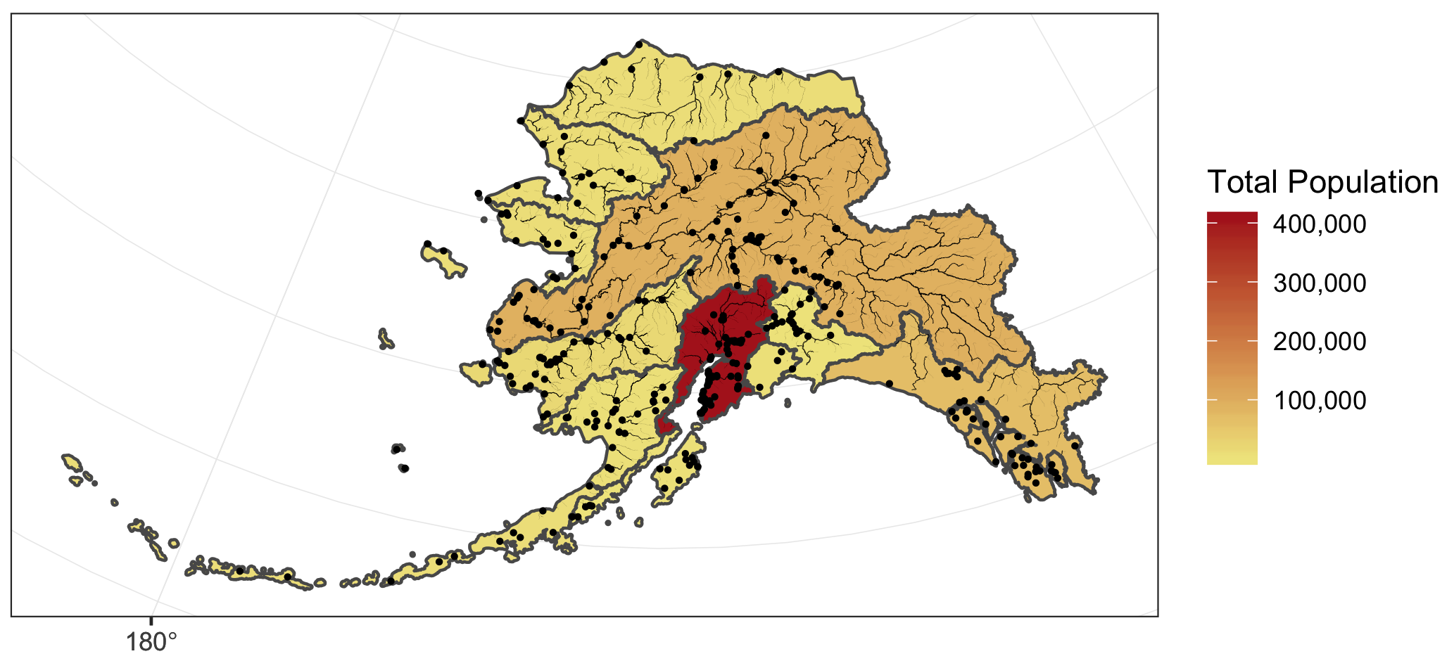
In this lesson, our goal is to use spatial data on Alaska regions and community populations to summarize population per region. From this, we will then create a map that shows regional populations, major rivers, and community locations:
3 About the Data
Most of the data used in this tutorial are simplified versions of real datasets available on the KNB Data Repository. We are using simplified datasets to ease the processing burden on all our computers since the original geospatial datasets are high-resolution. These simplified versions of the datasets may contain topological errors.
The spatial data we will be using to create the map are:
| Data | Original datasets |
|---|---|
| Alaska regional boundaries | Jared Kibele and Jeanette Clark. 2018. State of Alaska’s Salmon and People Regional Boundaries. Knowledge Network for Biocomplexity. doi:10.5063/F1125QWP. |
| Community locations and population | Jeanette Clark, Sharis Ochs, Derek Strong, and National Historic Geographic Information System. 2018. Languages used in Alaskan households, 1990-2015. Knowledge Network for Biocomplexity. doi:10.5063/F11G0JHX. |
| Alaska rivers | The rivers shapefile is a simplified version of Jared Kibele and Jeanette Clark. Rivers of Alaska grouped by SASAP region, 2018. Knowledge Network for Biocomplexity. doi:10.5063/F1SJ1HVW. |
3.1 Download the Data
Open your project training_{username}. We will download a simplified version of the Alaska regional boundaries dataset. Here are two methods: programmatic (for reproducibility) and manual (perhaps more intuitive?). If you are working on a server, the programmatic method is probably best, since you won’t have to later upload the downloaded file to the server.
Here is programmatic code to download the dataset from KNB into your current project, unzip it into a folder, and then delete the zip file. Copy and paste this into the console in Positron or RStudio to run it. Then check that your data folder has an ak_regions subfolder with some files.
out_dir <- here::here('data/ak_regions')

if(!dir.exists(out_dir)) {
    knb_url <- "https://dev.nceas.ucsb.edu/knb/d1/mn/v2/object/urn%3Auuid%3Aaceaecb2-1ce0-4d41-a839-d3607d32bb58"

    download.file(url = knb_url,
                  destfile = 'shapefile_demo_data.zip',
                  mode = 'wb')

    unzip('shapefile_demo_data.zip', exdir = out_dir)

    file.remove('shapefile_demo_data.zip')
}
TipInclude this in your script?
You could include this code in your script, so any time anyone runs it for the first time it automatically downloads the required data. This is great for reproducibility!
The code above includes a check if(!dir.exists(out_dir)): if a user already has this directory, presumably they’ve downloaded the data so the script does not need to re-download it!
Navigate to this dataset on KNB’s test site and download the zip folder.
- If on a local computer: unzip the contents of this file into a folder
data/ak_regionswithin your current project. - If on a server: Upload the zip folder to a
data/ak_regionsfolder in thetraining_{username}project. You don’t need to unzip the folder ahead of time, uploading will automatically unzip the folder.
ImportantAdd spatial data to
.gitignore
Spatial data are typically binary format files, and often quite large (> 5 MB), and therefore not well suited for Git tracking. Let’s add them to the .gitignore in the project root folder, by adding a line /data/ak_regions/.
If you include code to programmatically download the data (see above), then any collaborators will be able to automatically download the data to their own computers, so no need to worry about sharing the data files themselves.
4 Set Up a New Analysis
In your training_{username} project, create a new Quarto file.
- Title it “Working with Vector Spatial Data in R” and add any other information to the YAML header (author, date, format features).
- Save the file and name it “intro_to_vector_spatial.qmd”. You may wish to save it in the project root, or a scripts folder - your choice!
Delete any default text below the YAML header and set up a basic structure with Markdown headers:
- Setup
- Data Exploration
- Analysis
- Visualization
In the Setup section, attach the following libraries in a code chunk (perhaps with #| warning: false and #| message: false options).
5 Explore the Data
TipOptional: include code here for programmatic download
To enhance reproducibility for others interested in this analysis, include the code here to download the data from the original source (ideally, checking whether it has already been downloaded)!
5.1 Read In and Plot
sf reads most vector formats (shapefiles, GeoPackages, GeoJSON, etc.) with a single function. The result looks and behaves like a data.frame, with one special column called geometry that holds the spatial information.
Read in the shapefile of regional boundaries in Alaska using read_sf() and then create a basic plot of the data plot(). Here we’re adding a _sf suffix to our object name, to remind us that this is a Simple Features object with spatial information.
ak_rgns_sf <- read_sf(here("data/ak_regions/ak_regions_simp.shp"))When we plot the basic object, it shows us a mini plot for each attribute.
# quick plot
plot(ak_rgns_sf)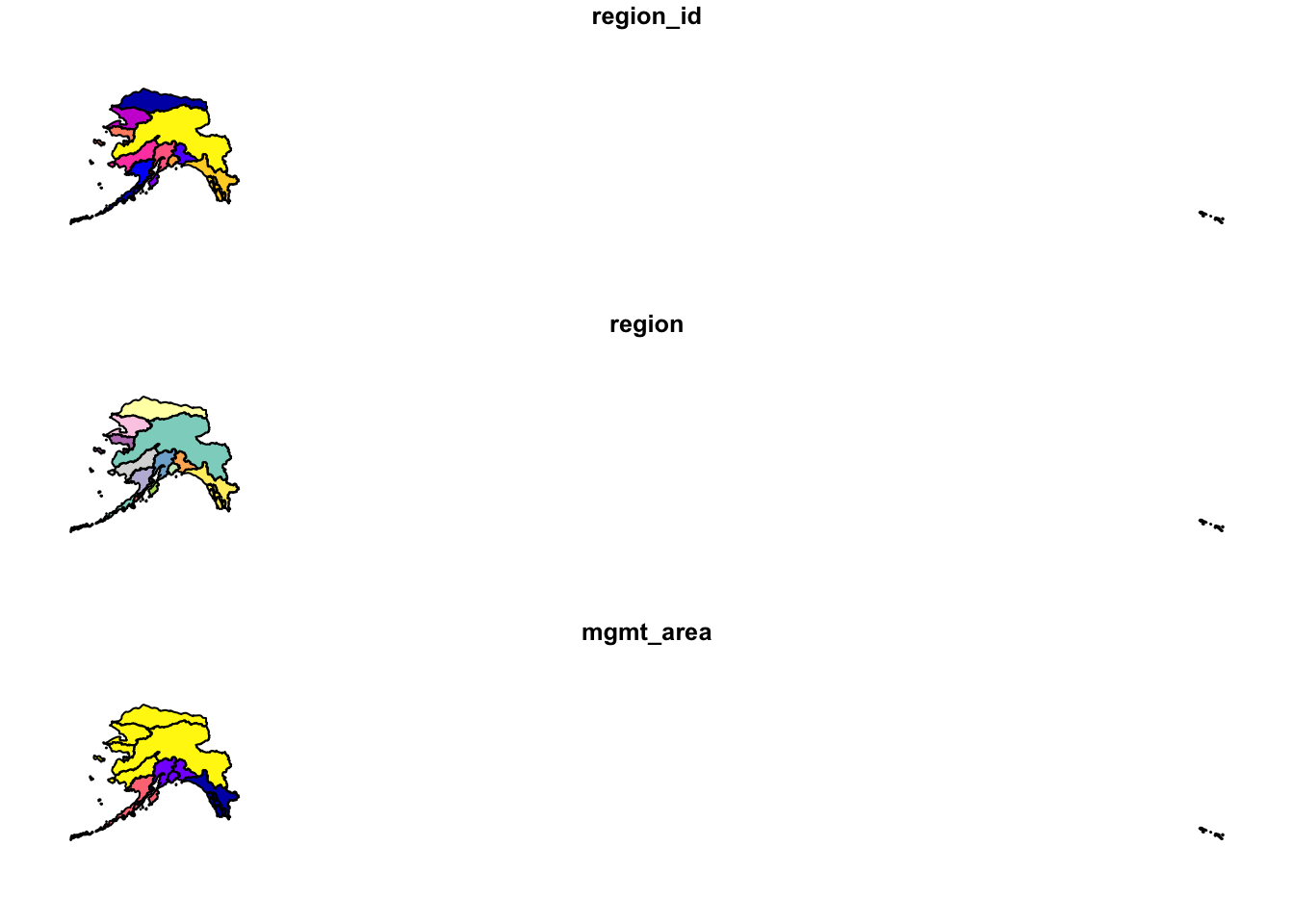
5.2 Coordinate Reference Systems (CRS)

Every spatial dataset has a coordinate reference system (CRS) that ties coordinates to locations on Earth. The CRS bundles two things:
- Datum — the reference ellipsoid (e.g., WGS84, NAD83)
- Projection — the math that flattens the ellipsoid onto a 2-D plane
When there’s no projection, you’re working in geographic coordinates (latitude/longitude). Check the CRS with st_crs():
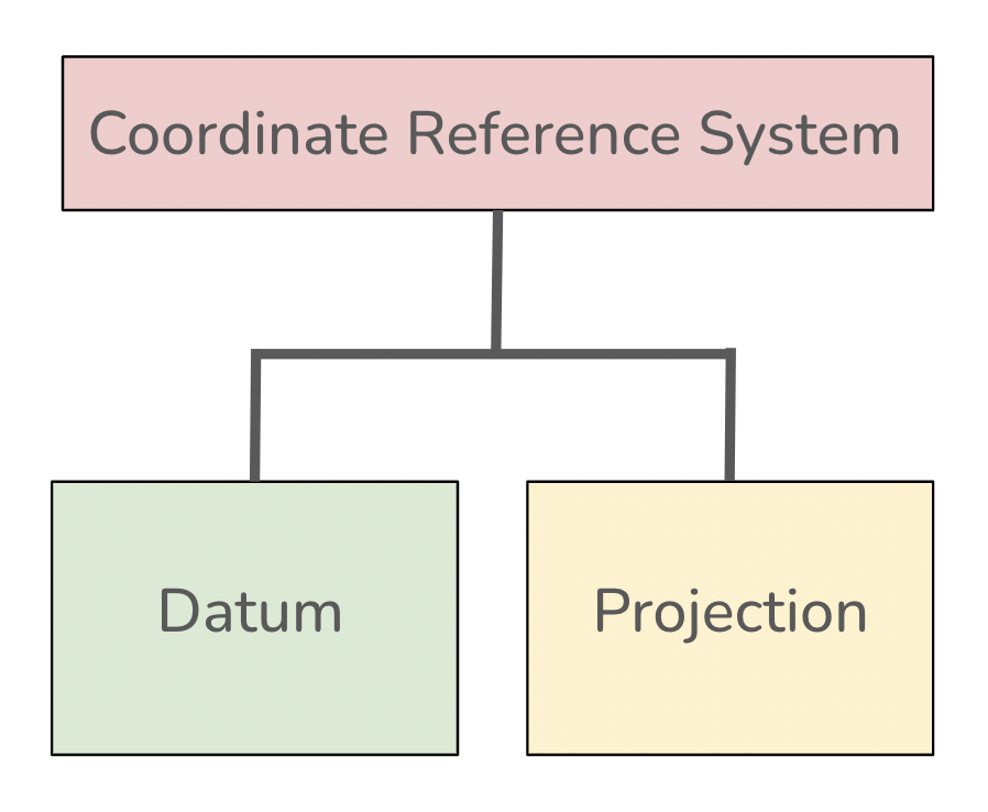
The datum is how you georeference your points (in 3 dimensions!) onto a spheroid, or the Earth. The Earth is not a perfect sphere and there are many ways to describe its shape. For example, is the Earth shaped like a lemon, lime, or orange? The shape, or datum, that you choose will depend on the scope of your project (for instance, local vs. global) and the specific locations.
The projection is how these points are mathematically transformed to represent the georeferenced point on a flat piece of paper. Since you will visualize a 3D object onto a 2D space, there will be some distortions depending on the projection that you choose. Analogously, how do you peel the fruit (representing the Earth) and flatten the peel?
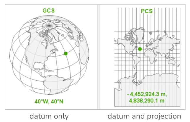
This blog post that explains these concepts in more detail with helpful diagrams and examples.
You can view what crs is set by using the function st_crs().
st_crs(ak_rgns_sf)Output (collapsed)
Coordinate Reference System:
  User input: WGS 84
  wkt:
GEOGCRS["WGS 84",
    DATUM["World Geodetic System 1984",
        ELLIPSOID["WGS 84",6378137,298.257223563,
            LENGTHUNIT["metre",1]]],
    PRIMEM["Greenwich",0,
        ANGLEUNIT["degree",0.0174532925199433]],
    CS[ellipsoidal,2],
        AXIS["latitude",north,
            ORDER[1],
            ANGLEUNIT["degree",0.0174532925199433]],
        AXIS["longitude",east,
            ORDER[2],
            ANGLEUNIT["degree",0.0174532925199433]],
    ID["EPSG",4326]]
This looks pretty confusing. Without getting into the details, that long string says that this data has a geographic coordinate system (WGS84) with no projection.
Every standard CRS has a short numeric EPSG code. The three you’ll use most in this lesson:
| EPSG | Name | Used for |
|---|---|---|
| 4326 | WGS84 | GPS coordinates, GeoJSON |
| 3338 | Alaska Albers | Alaskan data — equal-area, looks right |
| 3857 | Pseudo-Mercator | Web tile maps (Google, OpenStreetMap) |
Use st_transform() to reproject. Our data currently uses WGS84 (EPSG:4326), which distorts Alaska badly near the antimeridian. Let’s switch to Alaska Albers (here we’ll add the EPSG to our object name, along with _sf, as a reminder):
ak_rgns_3338_sf <- ak_rgns_sf %>%
    st_transform(crs = 3338)

# st_crs(ak_rgns_3338_sf) ### run in console to check
Output (collapsed)
Coordinate Reference System:
  User input: EPSG:3338
  wkt:
PROJCRS["NAD83 / Alaska Albers",
    BASEGEOGCRS["NAD83",
        DATUM["North American Datum 1983",
            ELLIPSOID["GRS 1980",6378137,298.257222101,
                LENGTHUNIT["metre",1]]],
        PRIMEM["Greenwich",0,
            ANGLEUNIT["degree",0.0174532925199433]],
        ID["EPSG",4269]],
    CONVERSION["Alaska Albers (meter)",
        METHOD["Albers Equal Area",
            ID["EPSG",9822]],
        PARAMETER["Latitude of false origin",50,
            ANGLEUNIT["degree",0.0174532925199433],
            ID["EPSG",8821]],
        PARAMETER["Longitude of false origin",-154,
            ANGLEUNIT["degree",0.0174532925199433],
            ID["EPSG",8822]],
        PARAMETER["Latitude of 1st standard parallel",55,
            ANGLEUNIT["degree",0.0174532925199433],
            ID["EPSG",8823]],
        PARAMETER["Latitude of 2nd standard parallel",65,
            ANGLEUNIT["degree",0.0174532925199433],
            ID["EPSG",8824]],
        PARAMETER["Easting at false origin",0,
            LENGTHUNIT["metre",1],
            ID["EPSG",8826]],
        PARAMETER["Northing at false origin",0,
            LENGTHUNIT["metre",1],
            ID["EPSG",8827]]],
    CS[Cartesian,2],
        AXIS["easting (X)",east,
            ORDER[1],
            LENGTHUNIT["metre",1]],
        AXIS["northing (Y)",north,
            ORDER[2],
            LENGTHUNIT["metre",1]],
    USAGE[
        SCOPE["Topographic mapping (small scale)."],
        AREA["United States (USA) - Alaska."],
        BBOX[51.3,172.42,71.4,-129.99]],
ID["EPSG",3338]]plot(ak_rgns_3338_sf)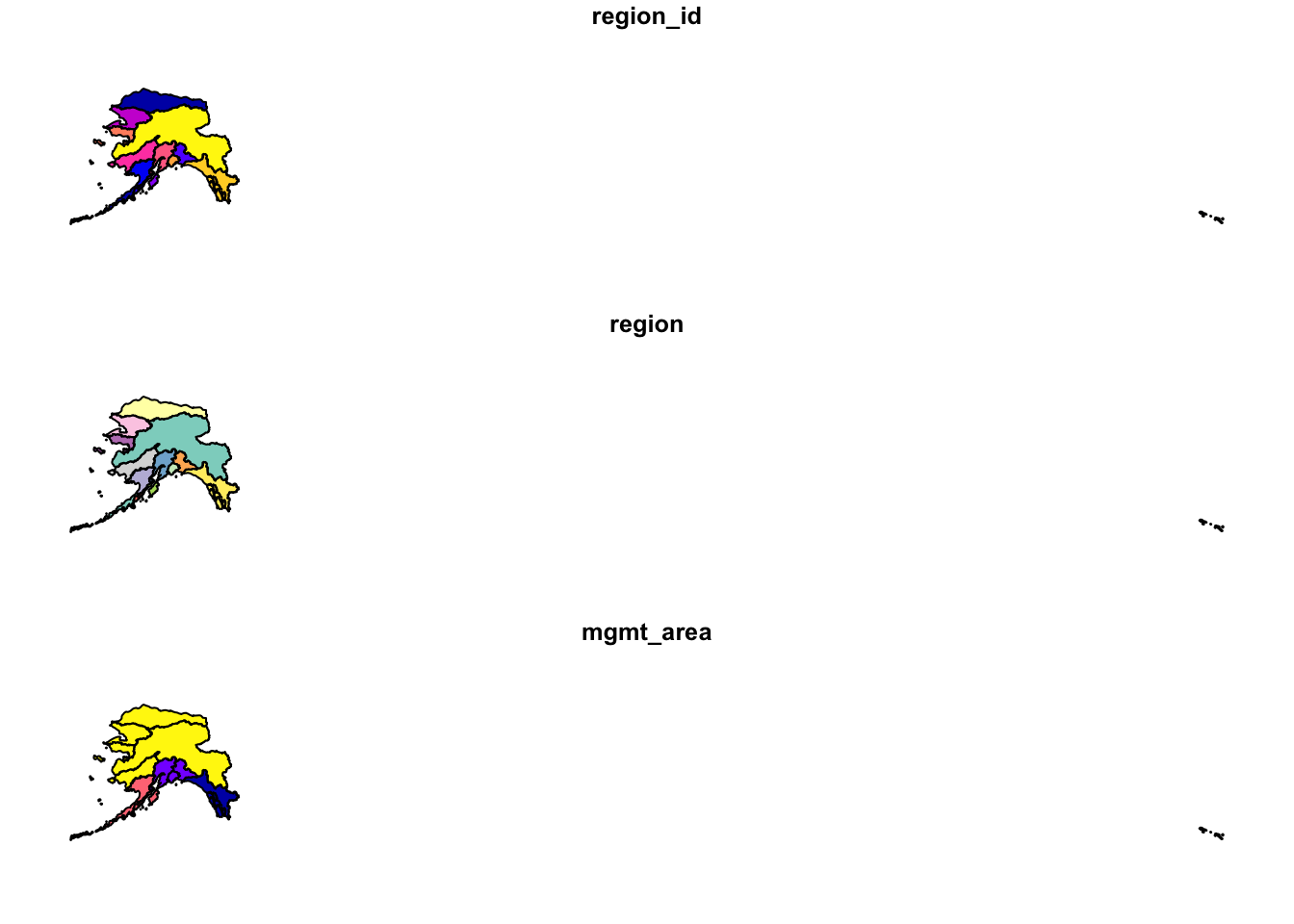
Much better!
6 sf & the Tidyverse
Examine the class of our spatial data using class().
class(ak_rgns_3338_sf)[1] "sf" "tbl_df" "tbl" "data.frame"sf objects should have (at least) two classes: sf and data.frame. Let’s look at their basic structure:
Output (collapsed)
Simple feature collection with 6 features and 3 fields
Geometry type: MULTIPOLYGON
Dimension:     XY
Bounding box:  xmin: -2175328 ymin: 405653 xmax: 773820 ymax: 2383770
Projected CRS: NAD83 / Alaska Albers
# A tibble: 6 × 4
  region_id region           mgmt_area                    geometry
      <int> <chr>                <dbl>          <MULTIPOLYGON [m]>
1         1 Aleutian Islands         3 (((-1156666 420855.1, -115…
2         2 Arctic                   4 (((571289.9 2143072, 56994…
3         3 Bristol Bay              3 (((-339688.6 973904.9, -33…
4         4 Chignik                  3 (((-114381.9 649966.8, -11…
5         5 Copper River             2 (((561012 1148301, 559393.…
6         6 Kodiak                   3 (((115112.5 983293, 113051…
Output (collapsed)
Rows: 13
Columns: 4
$ region_id <int> 1, 2, 3, 4, 5, 6, 7, 8, 9, 10, 11, 12, 13
$ region    <chr> "Aleutian Islands", "Arctic", "Bristol Bay", "…
$ mgmt_area <dbl> 3, 4, 3, 3, 2, 3, 4, 4, 2, 4, 2, 1, 4
$ geometry  <MULTIPOLYGON [m]> MULTIPOLYGON (((-1156666 42..., MULTIPOLYGON (…
Since our shapefile object has the data.frame class, all the usual dplyr and tidyr functions work on them, just as if we read in tabular data using read.csv() or read_csv().
But, unlike a typical data.frame, an sf object has an additional column typically named geometry that contains the spatial data. This geometry column is sticky - it will stick around even if you don’t explicitly ask for it. For example:
### select keeps `region` AND `geometry` automatically
ak_rgns_3338_sf %>%
    select(region) %>%
    head()
Output (collapsed)
Simple feature collection with 6 features and 1 field
Geometry type: MULTIPOLYGON
Dimension:     XY
Bounding box:  xmin: -2175328 ymin: 405653 xmax: 773820 ymax: 2383770
Projected CRS: NAD83 / Alaska Albers
# A tibble: 6 × 2
  region                                                  geometry
  <chr>                                         <MULTIPOLYGON [m]>
1 Aleutian Islands (((-1156666 420855.1, -1159837 417990.3, -1161…
2 Arctic           (((571289.9 2143072, 569941.5 2142691, 569158.…
3 Bristol Bay      (((-339688.6 973904.9, -339302 972297.3, -3392…
4 Chignik          (((-114381.9 649966.8, -112866.8 652065.8, -10…
5 Copper River     (((561012 1148301, 559393.7 1148169, 557797.7 …
6 Kodiak           (((115112.5 983293, 113051.3 982825.9, 110801.…
### filter() works exactly as expected!
ak_rgns_3338_sf %>%
filter(region %in% c("Arctic", "Kodiak"))- 1
-
Recall that
==is problematic if you’re testing whether a variable might match multiple values - use%in%for that situation!
Output (collapsed)
Simple feature collection with 2 features and 3 fields
Geometry type: MULTIPOLYGON
Dimension:     XY
Bounding box:  xmin: -497326.7 ymin: 704730.2 xmax: 706032.5 ymax: 2383770
Projected CRS: NAD83 / Alaska Albers
# A tibble: 2 × 4
  region_id region mgmt_area                              geometry
*     <int> <chr>      <dbl>                    <MULTIPOLYGON [m]>
1         2 Arctic         4 (((571289.9 2143072, 569941.5 214269…
2         6 Kodiak         3 (((115112.5 983293, 113051.3 982825.…
7 Spatial Joins
We can also use the sf package to create spatial joins, useful for when you want to utilize two spatial datasets together.
As an example, let’s explore the question: How many people live in each of these Alaska regions?
We have some population data that gives the population by city, not by region. To determine the population per region we will need to:
- Read in the population data from a
csvand turn it into ansfobject - Use a spatial join (
st_join()) to match each city to a region - Use
group_by()andsummarize()to calculate the total population by region - Save the resulting spatial object using
write_sf()
7.1 Download the Population Data
As for the vector spatial data, let’s download the population data either programmatically or manually. Here we are downloading the full dataset, not a simplified one. Save it as data/alaska_population.csv (NOT in the ak_regions folder).
Copy and paste this into the console in Positron or RStudio to run it. Then check your data folder for the file.
out_file <- here::here('data/alaska_population.csv')

if(!file.exists(out_file)) {
    pop_data_url <- "https://knb.ecoinformatics.org/knb/d1/mn/v2/object/urn%3Auuid%3A7fc6f6db-c5ea-426a-a743-1f2edafb43b8"

    download.file(url = pop_data_url,
                  destfile = out_file,
                  mode = 'w')
}
Navigate to this dataset on the KNB site and click the download button for the file called household_language.csv. (We’re only going to use the population data from this file)
- If on a local computer: Save it or move it into the current project as
data/alaska_population.csv. - If on a server: Upload the file to the
datafolder in thetraining_{username}project asdata/alaska_population.csv.
7.2 Read in Population Data
This dataset actually includes a lot more than just population by city - it also includes info on how many people in each city speak different languages. But for this example, we’ll just focus on the population column, using dplyr methods to filter for the most recent year of data (2015) and select the relevant columns.
Here we’ll add a _df suffix to remind us that this is just a regular data frame, not a spatial data frame. It does contain spatial variables (longitude and latitude), but as far as it knows, those are just numbers, not recognized as spatial geometry… yet!
pop_df <- read_csv(here("data/alaska_population.csv")) %>%
    filter(Year == 2015) %>%
    select(city, lat, lng, population = total) %>%
    drop_na()
7.3 Turn pop_df Into a Spatial Object
Our dataframe has lat long values, which we will use to turn our population data.frame into an sf object.
We can do this easily using the st_as_sf() function, which takes as arguments the coordinates and the crs. Although the CRS isn’t noted explicitly in the file, let’s assume that the lat long coordinates are in WGS84, or EPSG:4326, a very common CRS for lat-long data.
Note that we’re adding a _sf suffix to our new object, because now it is a Simple Features spatial data frame!
pop_4326_sf <- st_as_sf(pop_df,
coords = c('lng', 'lat'),
crs = 4326,
remove = FALSE)- 1
- This refers to the associated column names in the dataframe; x is longitude, y is latitude.
- 2
-
remove = FALSEoverrides the default to drop the longitude/latitude columns; we’ll need those later!
Note the geometry column for this contains points!
head(pop_4326_sf)Output (collapsed)
Simple feature collection with 6 features and 4 fields
Geometry type: POINT
Dimension:     XY
Bounding box:  xmin: -176.6581 ymin: 51.88 xmax: -154.1703 ymax: 62.68889
Geodetic CRS:  WGS 84
# A tibble: 6 × 5
  city       lat   lng population             geometry
  <chr>    <dbl> <dbl>      <dbl>          <POINT [°]>
1 Adak      51.9 -177.        122    (-176.6581 51.88)
2 Akhiok    56.9 -154.         84 (-154.1703 56.94556)
3 Akiachak  60.9 -161.        562 (-161.4314 60.90944)
4 Akiak     60.9 -161.        399 (-161.2139 60.91222)
5 Akutan    54.1 -166.        899 (-165.7731 54.13556)
6 Alakanuk  62.7 -165.        777 (-164.6153 62.68889)
7.4 Join Population Data with Alaska Regions
Now we can do our spatial join! We specify a “geometric predicate function” to determine how to match geometries - e.g., st_intersects, st_within, st_crosses, st_is_within_distance - in the join argument. The geometric predicate function you use will depend on what kind of operation you want to do, and the geometries of your shapefiles.
In this case, we want to find what region (polygon) each city (point) falls within, so we will use st_within.
NOTE: Both geometries must use the same CRS - otherwise we get an error: st_crs(x) == st_crs(y) is not TRUE. So first we transform our population data from WGS84 (4326) to Alaska Albers (3338)
pop_3338_sf <- st_transform(pop_4326_sf,
                            crs = 3338)

pop_joined_sf <- st_join(pop_3338_sf,
                         ak_rgns_3338_sf,
join = st_within)head(pop_joined_sf)Output (collapsed)
Simple feature collection with 6 features and 7 fields
Geometry type: POINT
Dimension:     XY
Bounding box:  xmin: -1537925 ymin: 472626.9 xmax: -10340.71 ymax: 1456223
Projected CRS: NAD83 / Alaska Albers
# A tibble: 6 × 8
  city    lat   lng population             geometry region_id
  <chr> <dbl> <dbl>      <dbl>          <POINT [m]>     <int>
1 Adak   51.9 -177.        122  (-1537925 472626.9)         1
2 Akhi…  56.9 -154.         84 (-10340.71 770998.4)         6
3 Akia…  60.9 -161.        562  (-400885.5 1236460)         8
4 Akiak  60.9 -161.        399  (-389165.7 1235475)         8
5 Akut…  54.1 -166.        899 (-766425.7 526057.8)         1
6 Alak…  62.7 -165.        777  (-539724.9 1456223)        13
# ℹ 2 more variables: region <chr>, mgmt_area <dbl>
Each point from the city population data now includes a region name from the Alaska regions data. Note, only the point geometry is kept here! If we swapped the order of the datasets, we would keep the region geometry instead.
NoteExploring types of join predicates
Other useful join predicates include st_intersects (any overlap), st_crosses (lines crossing polygons), and st_is_within_distance (proximity). See ?st_within for the full list.
7.5 Calculate Total Population by Region
Next we compute the total population for each region. In this case, we want to do a group_by() and summarize() as if this were a regular data.frame, without the spatial information - otherwise all of our point geometries would be included in the aggregation, which is not what we want. We remove the sticky geometry using st_drop_geometry(). Here we’re going to add a _df suffix because it’s no longer a spatial data frame.
pop_rgn_df <- pop_joined_sf %>%
    st_drop_geometry() %>%
    group_by(region) %>%
summarize(total_pop = sum(population))head(pop_rgn_df)Output (collapsed)
# A tibble: 6 × 2
  region           total_pop
  <chr>                <dbl>
1 Aleutian Islands      8840
2 Arctic                8419
3 Bristol Bay           6947
4 Chignik                311
5 Cook Inlet          408254
6 Copper River          2294
And then we use a regular left_join() to connect the (non-spatial) population dataframe back to the Alaska region spatial dataframe.
pop_rgn_3338_sf <- left_join(ak_rgns_3338_sf,
                             pop_rgn_df,
                             by = "region")

### plot to check
plot(pop_rgn_3338_sf["total_pop"])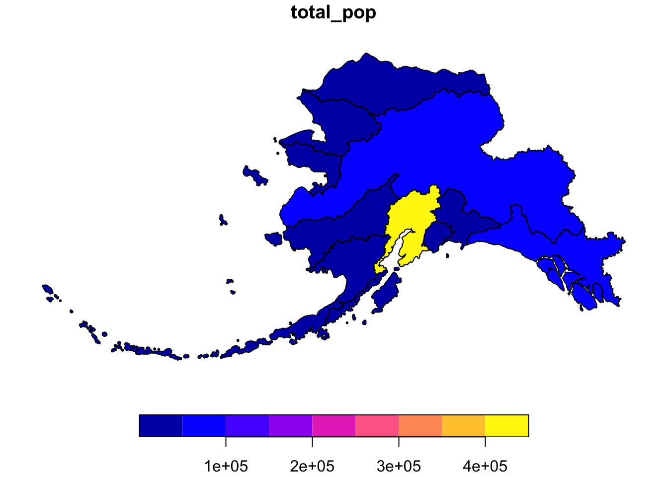
So far, we have learned how to use sf and dplyr to use a spatial join on two datasets and calculate a summary metric from the result of that join.
7.6 Dissolving Geometries with group_by() %>% summarize()
Say we want to calculate the population by Alaska management area, each of which contains multiple regions, instead of at the region level.
pop_mgmt_3338_sf <- pop_rgn_3338_sf %>%
    group_by(mgmt_area) %>%
    summarize(total_pop = sum(total_pop))

plot(pop_mgmt_3338_sf["total_pop"])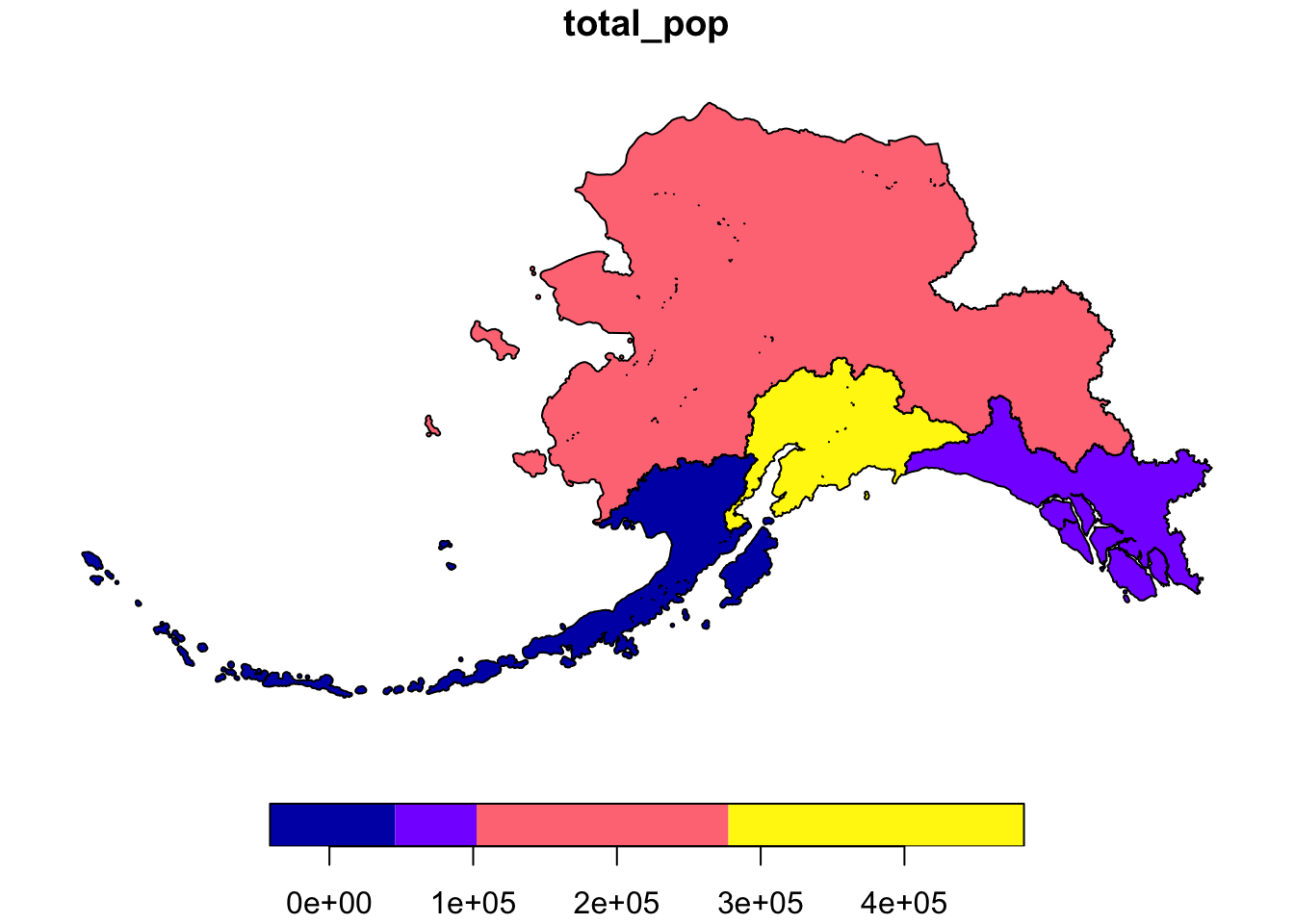
Notice that the region geometries were combined into a single polygon for each management area. (The little irregular dots are a result of having simplified our vector data to reduce file sizes and computation time for this lesson).
Set the argument do_union = FALSE inside summarize() to keep the original region polygons instead of dissolving them.
Note
sf and tidyverse best practices
The group_by() and summarize() functions can also be used on sf objects to summarize within a dataset and combine geometries. Many of the tidyverse functions have methods specific for sf objects, some of which have additional arguments that wouldn’t be relevant to the data.frame methods. You can run ?sf::tidyverse to get documentation on the tidyverse sf methods.
7.7 Save the Spatial Object to a New File
Save the spatial object using write_sf() and specifying the filename. The file extension controls the format (.shp = ESRI Shapefile, .gpkg = GeoPackage, .geojson = GeoJSON). GeoPackage is generally preferred over Shapefile for new work — it’s a single file, is filesize efficient, supports long field names, and handles multiple layers.
write_sf(pop_rgn_3338_sf, here("data/ak_regions_population.gpkg"))8 Visualize Static Maps with ggplot2
ggplot2 has integrated functionality to plot sf objects using geom_sf(), using the information from the geometry column.
We can plot any sf object using geom_sf:
ggplot(pop_rgn_3338_sf) +
    geom_sf(aes(fill = total_pop)) +
    labs(fill = "Total Population") +
    scale_fill_continuous(low = "khaki", high =  "firebrick") +
    theme_bw()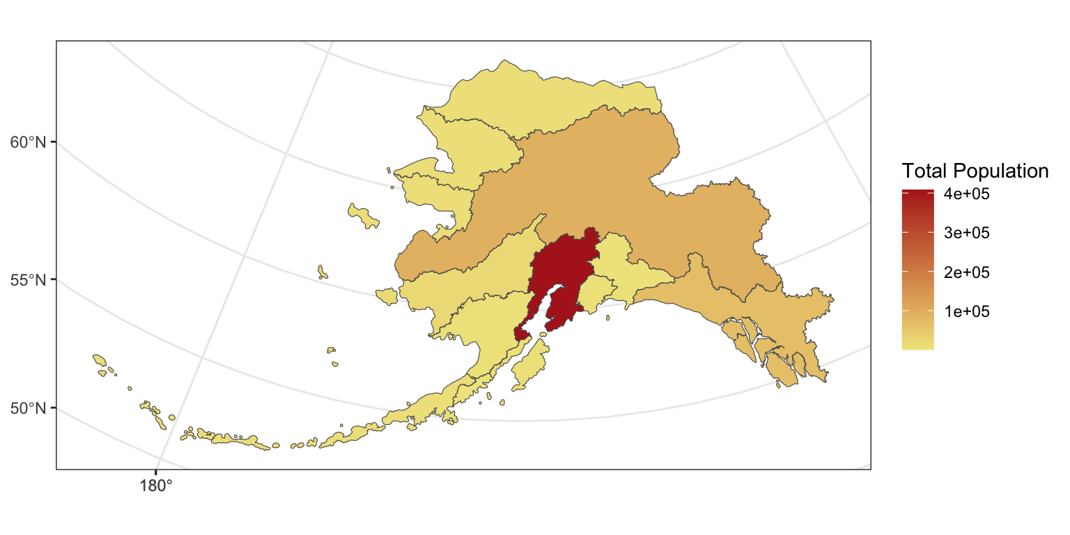
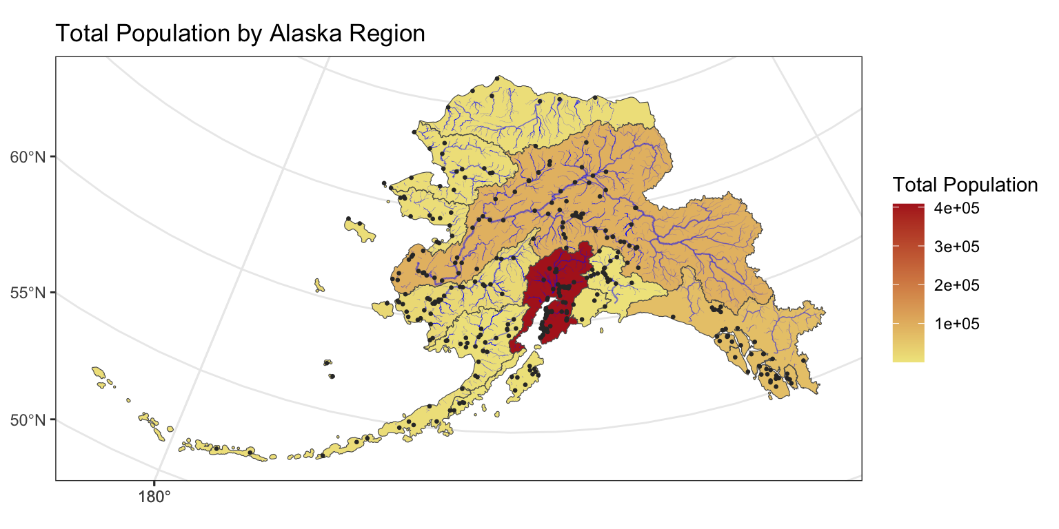
Layer multiple geometries exactly like regular ggplot2. Here it is best to separately assign each data = and mapping = aes() inside each geom_sf call. Later geoms are visually stacked on top of earlier geoms. Let’s read in and add a simplified rivers dataset to the plot (already downloaded with the Alaska regions, and already in EPSG:3338), along with cities from our pop_3338_sf data:
rivers_3338_sf <- read_sf(here("data/ak_regions/ak_rivers_simp.shp"))ggplot() +
geom_sf(data = pop_rgn_3338_sf,
mapping = aes(fill = total_pop)) +
geom_sf(data = rivers_3338_sf,
aes(linewidth = StrOrder),
color = 'blue', alpha = .5) +
scale_linewidth(range = c(0.05, 0.5),
guide = "none") +
geom_sf(data = pop_3338_sf, size = 0.5, color = 'grey20') +
labs(title = "Total Population by Alaska Region",
fill = "Total Population") +
scale_fill_continuous(low = "khaki",
high = "firebrick") +
theme_bw() - 1
- Stream order is aesthetically mapped to river line thickness - bigger rivers, thicker lines!
8.1 Incorporate Base Maps Into Static Maps
The ggspatial package has a function that can add tile layers from a few predefined tile sources like OpenStreetMap. Making sure that the tiles will plot correctly can be a finicky, so we will reproject our population data into the OpenStreetMap projection, Pseudo-Mercator (EPSG 3857), first.
Then we will add ggspatial::annotation_map_tile() function to our plot to add a base map under our map (higher zoom argument means finer detail but slower loading time). We will also zoom in on Anchorage to show more detail of the map tile!
pop_3857_sf <- st_transform(pop_3338_sf,
crs = 3857)ggplot(data = pop_3857_sf) +
ggspatial::annotation_map_tile(type = "osm", zoom = 6, progress = 'none') +
# higher zoom values are more detailed
geom_sf(aes(color = population),
fill = NA) +
coord_sf(xlim = c(-16900000, -16300000), ylim = c(8400000, 9000000)) +
scale_color_continuous(low = "darkkhaki",
high = "firebrick")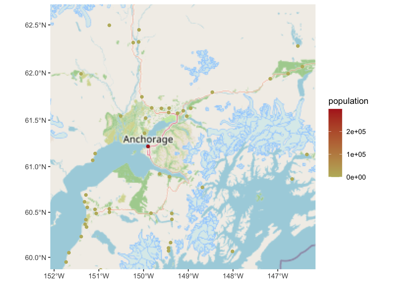
TipZoom in with
coord_sf()
coord_sf() lets you zoom into a bounding box without subsetting your data:
coord_sf(xlim = c(-500000, 600000), ylim = c(900000, 2000000))
9 Visualize Interactive Maps With leaflet
We can also make an interactive map from our data above using leaflet.
leaflet builds interactive, pannable/zoomable maps. It handles reprojection internally, but expects data in WGS84 (EPSG:4326). If you want to display in a custom projection (like Alaska Albers), you need leaflet.extras or the proj4leaflet plugin — for most use cases WGS84 is fine.
9.1 Create Basic leaflet Map
Since leaflet requires that we use an unprojected coordinate system, let’s use st_transform() get our joined data again to get back to WGS84.
pop_rgn_4326_sf <- pop_rgn_3338_sf %>%
    st_transform(crs = 4326)
Like ggplot we first initialize the plot with leaflet() and then add features (basemaps, polygons, points) and themes (colors, labels, legends). Note, Leaflet layers are added using a pipe (%>% or |>) instead of a plus +.
### set up a palette based on our colors
pal <- colorNumeric(palette = "Reds", domain = pop_rgn_4326_sf$total_pop)
pop_rgn_map <- leaflet(data = pop_rgn_4326_sf) %>%
addProviderTiles("CartoDB.Positron") %>%
addPolygons(
fillColor = ~pal(total_pop),
fillOpacity = 0.8,
color = "white",
weight = 1,
label = ~paste0(region, ": ", total_pop)
) %>%
addLegend(
position = "bottomleft",
pal = pal,
values = ~total_pop,
title = "Total Population"
)
pop_rgn_map- 1
- Add a basemap
- 2
-
Add polygons; here we are using the default data assigned inside
leaflet()
9.2 Add Cities and Zoom In
We can also add the individual communities, with popup labels showing their population, on top of that.
pop_rgn_map <- pop_rgn_map %>%
addCircleMarkers(
data = pop_4326_sf,
radius = ~ log(population / 500),
fillColor = "gray",
fillOpacity = 1,
weight = 0.25,
color = "black",
label = ~ paste0(pop_4326_sf$city,
", population ",
pop_4326_sf$population)
) - 1
- On top of everything in the previous map, we can keep adding layers directly
- 2
-
This overrides the default data from
leaflet()to instead use the city points:pop_4326_sf - 3
- This is an arbitrary scaling of point size
- 4
- Tooltip labels - hover over a city point to see the information!
Before we plot, let’s zoom in two ways: focusing on a point and zoom level, and focusing on a bounding box.
Here we focuson the Anchorage area using setView(), which takes a longitude, latitude, and zoom level (higher zoom = more detail). We can simply add it to the end of our map object. Here we pull the lat/long for Anchorage from our population data frame, but you could also just look it up and hardcode it.
anch_latlong <- pop_df %>%
    filter(city == "Anchorage") %>%
    select(lat, lng)
anch_latlong
# A tibble: 1 × 2
lat lng
<dbl> <dbl>
1 61.2 -150.pop_rgn_map %>%
setView(lng = anch_latlong$lng, lat = anch_latlong$lat, zoom = 5)Alternatively, we can zoom in on a bounding box using fitBounds(), which takes the longitude and latitude of two opposite corner points. Here we use st_bbox() to get those coordinates from our spatial dataframe of population by region, but there seems to be a bug if we pass those to fitBounds() as is. Here we coerce the bounding box coordinates to a format that fitBounds() can use (as.numeric), but you could also just look up the lat/long for the corners and hardcode them.
ak_bbox <- st_bbox(pop_4326_sf) %>%
    as.numeric()
pop_rgn_map %>%
    fitBounds(lng1 = ak_bbox[1], lat1 = ak_bbox[2],
              lng2 = ak_bbox[3], lat2 = ak_bbox[4])
10 Geometry Operations (Going Further)
The sf package includes a full suite of geometric operations beyond joins. A few you’ll reach for often:
| Function | What it does |
|---|---|
st_buffer(x, dist) |
Create a buffer zone around features |
st_intersection(x, y) |
Clip x to the overlap with y |
st_union(x) |
Merge all features into one |
st_distance(x, y) |
Compute pairwise distances |
st_area(x) |
Calculate polygon area |
st_centroid(x) |
Get the centroid point of each feature |
st_bbox(x) |
Return the bounding box |
Example — buffer cities by 50 km and find which regions they intersect:
city_buffers <- pop_3338_sf |>
  st_buffer(dist = 50000)   ### distance in CRS units (meters for EPSG:3338)

buffered_rgns <- st_intersection(city_buffers, ak_rgns_3338_sf)

plot(buffered_rgns %>% select(region))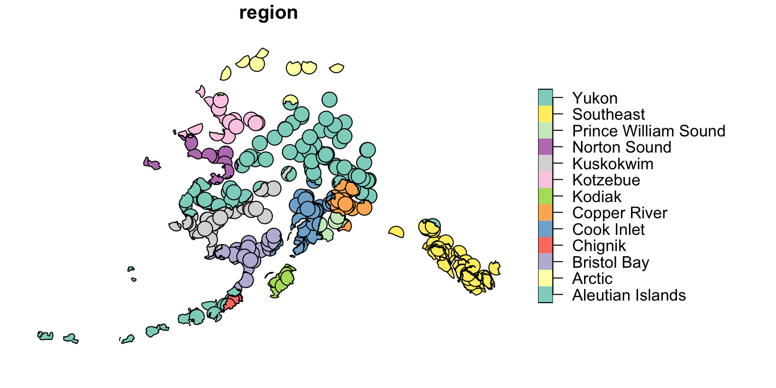
11 More Spatial Resources
Here are some more great resources and tutorials for a deeper dive into working with spatial data in R:
- sf github repo - scroll down to the README
- Geocomputation with R - online book on geographic data analysis, visualization, and modeling
- Spatial Data Science with R and
terra- online book focusing on raster spatial data using theterraR package - Spatial Data Science - another online book, written by the people who created the
sfpackage - mapping-fall-foliage-with-sf - an older resource, but a fun example of using
sfandggplot2to map and animate progress of fall foliage, for all you leaf-peepers out there