Publishing to the Web – 2026 Delta Synthesis Working Groups week 2 (April 2026)

Learning Objectives

After completing this session, you will be able to:

Publish a Quarto analysis to the web using Git and GitHub Pages
Create a multi-page site with a landing page that correctly links to a content page
Add interactive tables and maps to an HTML document using DT and leaflet
Follow the complete author → render → commit → push → verify publishing workflow

1 Introduction

Everything you’ve done so far using R – your wrangled data and visualizations – lives on your laptop. This session changes that: we’ll take the analysis you built in the previous lesson and publish it as a live, interactive website anyone can visit by URL.

Quarto’s HTML output format unlocks capabilities that static formats (PDF, Word) can’t match:

Interactive plots you can zoom, hover, and filter (you already made one with ggplotly)
Sortable, searchable tables that let readers explore data directly in the browser
Interactive maps readers can pan, zoom, and click

These elements are powered by JavaScript libraries (plotly.js, DataTables, and Leaflet.js) that R packages ggplotly(), DT, and leaflet make it easy for you to use in R. They work because web browsers run JavaScript; HTML is the right output format when you want to share interactive analyses.

A published example

Here is an example of a published data analysis site built with these same tools. Notice the interactive maps, the clean landing page, and how individual analyses are linked from it. That is the structure we will build today.

2 Set Up GitHub Pages

Steps

Make sure you are in your training_{USERNAME} project
Create a new Quarto document called index.qmd at the top level of your project
1. File → New File → Quarto Document
2. Set the title (e.g., "Delta Socioecological Monitoring"), keep Default Output Format as HTML, click OK
3. If your IDE added default template content below the YAML header, delete it
4. Add a brief description and a placeholder for your analyses:
```
Welcome to my Delta socioecological monitoring analysis.

## Course Analyses

- Data Visualization (link coming soon)
```
Save as index.qmd. Be sure to use this exact name, all lowercase. Web servers return index.html by default when no specific file is requested, so this name matters.
Render index.qmd and observe the new index.html in the same directory
Commit both index.qmd and index.html with a descriptive message, and push to GitHub
- If an index_files/ folder appears, commit it too – it holds supporting files for the HTML
In your browser, go to your GitHub repo → Settings → Pages
1. Keep Source as “Deploy from a branch”
2. Change Branch from “None” to main, keep folder as / (root), click Save
3. The message changes to “Your GitHub Pages site is currently being built from the main branch”

GitHub Pages follows a URL convention based on your username and repository name:

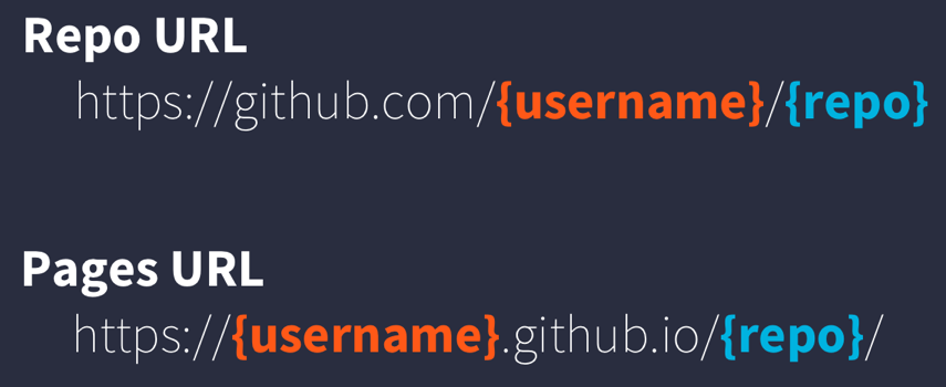
Note that it changes from github.com to github.io.

Visit https://{username}.github.io/{repo_name}/ (note the trailing /)
It may take a minute or two on first setup; refresh if you get a 404 error

Now make a small edit to confirm the full publish cycle works:

Update your published page

Add the text “Under construction” somewhere in index.qmd
Render index.qmd
Git workflow: Stage → Commit → Pull → Push
Wait ~1 minute, then revisit https://{username}.github.io/{repo_name}/ and confirm the change appears

3 Link Your Content Page

Now let’s connect your landing page to the visualization analysis you built in the previous session.

Relative paths

When linking between pages in your site, use a relative path from the linking file to the target file. Your index.qmd is at the repo root, and your visualization notebook is in a notebooks/ subfolder, so the correct link looks like this:

[Data Visualization](notebooks/data-visualization.html)

Common mistakes and what goes wrong:

Path	Problem
`notebooks/data-visualization.html`	✓ correct
`data-visualization.html`	✗ missing subfolder → 404
`notebooks/Data-Visualization.html`	✗ wrong case → 404 on case-sensitive servers
`notebooks/data-visualization.qmd`	✗ links to source, not rendered output

A 404 error (“Not Found”) means the browser cannot find the file at the path you gave it. Getting the path exactly right is one of the most common publishing stumbling blocks.

Exercise

Part 1: Trigger a broken link on purpose

In index.qmd, replace the placeholder with a link using a deliberately wrong path (missing the subfolder):

## Course Analyses

- [Data Visualization](data-visualization.html)

Render index.qmd, commit, push, then visit your live site and click the link. Observe the 404.

Part 2: Fix the link

Update the path to include the notebooks/ subfolder:

## Course Analyses

- [Data Visualization](notebooks/data-visualization.html)

Make sure notebooks/data-visualization.qmd has been rendered (so notebooks/data-visualization.html exists) and both files are committed. Render index.qmd, commit, push, and verify the link works on the live site.

4 Add Interactive Elements

Quarto’s HTML output format supports interactive elements powered by JavaScript, such as tables that users can sort and search, and maps they can pan and zoom. We’ll add two of these to notebooks/data-visualization.qmd: a searchable table using DT and an interactive map using leaflet.

Open notebooks/data-visualization.qmd and add the following to your setup chunk and then at the end of the document.

4.1 Setup

Add these packages to your setup chunk (or create one at the top of the document if you don’t have one yet):

```{r}
#| message: false
#| warning: false
library(readr)
library(here)
library(dplyr)
library(tidyr)
library(janitor)
library(DT)
library(leaflet)
```

The examples below use a daily_visits_loc data frame derived from the Delta socioecological monitoring dataset. Add this code after your setup chunk if you don’t already have it:

```{r}
delta_visits_raw <- read_csv(here("data/Socioecological_monitoring_data.csv"),
                             show_col_types = FALSE)

daily_visits_loc <- delta_visits_raw %>%
  janitor::clean_names() %>%
  tidyr::pivot_longer(
    cols      = c(sm_boat, med_boat, lrg_boat, bank_angler, scientist, cars),
    names_to  = "visitor_type",
    values_to = "quantity"
  ) %>%
  dplyr::rename(restore_loc = eco_restore_approximate_location) %>%
  dplyr::select(-notes) %>%
  dplyr::group_by(restore_loc, date, visitor_type) %>%
  dplyr::summarize(daily_visits = sum(quantity), .groups = "drop")
```

4.2 Interactive Table with `DT`

DT is an R package that wraps the DataTables JavaScript library, producing tables that readers can sort, search, and page through directly in the browser.

Add a new section:

## Interactive Table

```{r}
DT::datatable(
  daily_visits_loc,
  caption  = "Daily visitor counts at Delta restoration sites",
  colnames = c("Location", "Date", "Visitor type", "Daily visits"),
  options  = list(pageLength = 10)
)
```

Render the document and try sorting by column, searching for a specific location or visitor type, and paging through results.

Useful datatable() options

The options list accepts standard DataTables options. A few worth knowing:

pageLength: default number of rows shown
dom: controls which UI controls appear (search box, pagination, info, etc.)
columnDefs: per-column formatting (width, sorting, visibility)

See ?DT::datatable or the DT documentation for the full reference.

4.3 Interactive Map with `leaflet`

leaflet wraps the Leaflet.js JavaScript library for interactive maps. Its syntax is similar to ggplot2 in that you build up a map by adding layers, but it uses the pipe operator %>% rather than +.

We can pull the unique restoration site locations directly from the data we already loaded. Add this to your document:

## Interactive Map

```{r}
restoration_sites <- delta_visits_raw %>%
  janitor::clean_names() %>%
  distinct(restore_loc = eco_restore_approximate_location,
           latitude, longitude) %>%
  drop_na(latitude, longitude)

leaflet(restoration_sites) %>%
  addTiles() %>%
  addMarkers(
    lng   = ~longitude,
    lat   = ~latitude,
    popup = ~restore_loc
  )
```

Render the document, then pan the map, zoom in, and click a marker to see the popup.

Circle markers and color

For more control over marker appearance, use addCircleMarkers() instead of addMarkers():

leaflet(restoration_sites) %>%
  addTiles() %>%
  addCircleMarkers(
    lng         = ~longitude,
    lat         = ~latitude,
    popup       = ~restore_loc,
    radius      = 8,
    fillColor   = "steelblue",
    fillOpacity = 0.8,
    stroke      = FALSE
  )

As an extension exercise, try joining restoration_sites with total visit counts from daily_visits_loc and mapping fillColor to visit volume.

6 What’s Next

In this module, we published individual HTML pages linked from a landing page. A natural next step might be a proper Quarto website. This is a multi-page site where navigation, themes, and shared settings are configured in a single _quarto.yml file, giving you a consistent navigation bar across all pages.

For truly dynamic content that responds to user input in real time (e.g., filtering data on the fly, running models), look into Shiny, an R framework for building interactive web applications backed by a live R session.

Self-contained HTML files

If you want to share a single HTML file that works without a web server (e.g., via email), add this to your YAML header:

format:
  html:
    embed-resources: true

This bundles all JavaScript, CSS, and images into the HTML file itself. The trade-off is a larger file size; for sharing via URL, omitting embed-resources: true produces smaller, faster-loading pages.

7 Resources

Quarto Websites - documentation for building multi-page sites with shared navigation and _quarto.yml
GitHub Pages documentation - details about custom domains, build workflows, and more
DT package documentation - a full reference for interactive table options
Leaflet for R - a comprehensive guide including polygons, WMS tiles, and color scales