After completing this session, you will be able to:
- Describe the three principles of tidy data in terms of variables, observations, and values
- Identify common violations of tidy data principles and how to fix them
- Explain the concept of data normalization and how it supports reproducible analysis
- following best practices to format data tables’ content,
- relating tables following relational data models principles, and
- understanding how to perform table joins.
What is tidy data?
Tidy data is a standardized way of organizing data tables that allows us to manage and analyze data efficiently, because it makes it straightforward to understand the corresponding variable and observation of each value. The tidy data principles are:
- Every column is a single variable.
- Every row is a single observation.
- Every cell is a single value.
- Tidy data is not language or tool specific.
- Tidy data is not an R thing.
- Tidy data is not a
tidyverse thing.
Tidy Data is a way to organize data that will make life easier for people working with data.
(Allison Horst & Julia Lowndes)
Values, variables, observations, and entities
First, let’s get acquainted with our building blocks.
| Variable |
A characteristic that is being measured, counted or described with data. Example: car type, salinity, year, height, mass. |
| Observation |
A single “data point” for which the measure, count or description of one or more variables is recorded. Example: If you are collecting variables height, species, and location of plants, then each plant is an observation. |
| Value |
The record measured, count or description of a variable. Example: 3 ft |
| Entity |
Each type of observation is an entity. Example: If you are collecting variables height, species, and location and site name of plants and where they are observed, then plants is an entity and site is an entity. |
Tidy Data Principles
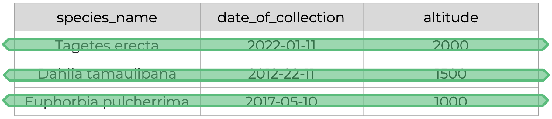
How are tidy data principles evident in this simple example? 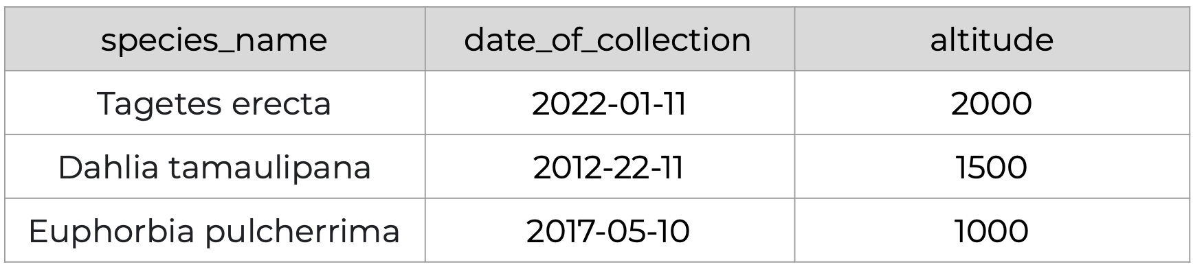
Principle 1: Every column is a single variable.
Principle 2: Every row is a single observation.
Principle 3: Every cell is a single value.
Recognizing untidy data
Anything that does not follow the three tidy data principles is untidy data. There are many ways in which data can become untidy, some can be noticed right away, while others are more subtle. In this slide deck we will look at some examples of common untidy data situations.
Full Screen
Why Tidy Data?
- Efficiency: A standardized format designed for computer readability means less effort in reshaping data, and reduced chance of introducing errors.
- Generalizability: Tools and techniques built for preparing one tidy data set can readily be applied to other tidy datasets.
- Scalability: Tidy datasets can easily be updated with new data, linked to other datasets, and managed as they scale in size.
- Collaboration: Makes it easier to work with others through a shared understanding of tidy data best practices.
“There is a specific advantage to placing varables in columns becasuse it allows R’s vectorized nature to shine. …most buit-in R functions work with vectors of values. That makes transforming tidy data feel particularly natural. (R for Data Science by Grolemund and Wickham)
Data Normalization
What is data normalization?
Data normalization is the process of eliminating redundancy in datasets to simplify query, analysis, storing, and maintenance.
In such normalized data we organize data so that :
- Each table follows the tidy data principles
- We have separate tables for each type of entity measured
- Observations (rows) are all unique
- Each column represents either an identifying variable or a measured variable
In denormalized data, observations about different entities are combined. A good indication that a data table is denormalized and needs normalization is seeing the same column values repeated across multiple rows.
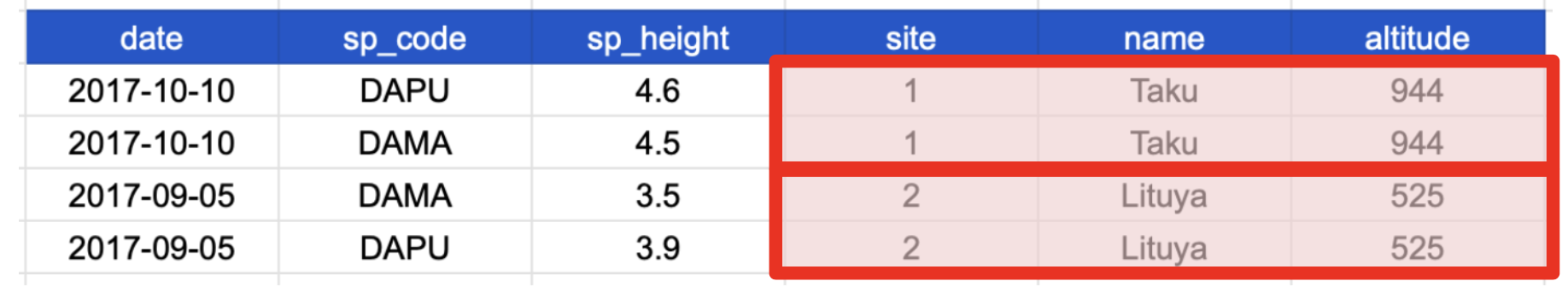
Examine this sample of data. Do you see any repeated values or redundancy?
Repeated row values may indicate that observations for different entities are combined.
- 1st entity: individual plants found at that site (
sp_code, sp_height)
- 2nd entity: sites at which the plants were observed (
site, name, altitude)
Once we know the name, altitude for one site for one species, it is redundant to repeat all that information for the next species. We can recreate that information just knowing the site ID number.
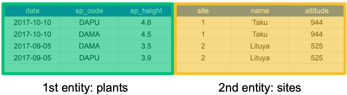
We can normalize this data by separating the information for the two entities, plant species and site, into two different tables
If we use this information to normalize our data, we should end up with:
- one tidy table for each entity observed, and
- additional columns for identifying variables (such as site ID).
Here’s how our normalized data would look; note the site identifying variable shows up in both tables:
Notice that each table also satisfies the tidy data principles.
Normalizing data by separating it into multiple tables often makes researchers really uncomfortable. This is understandable! The person who designed this study collected all of these measurements for a reason - so that they could analyze the measurements together. Now that our site and plant information are in separate tables, how would we use site altitude as a predictor variable for species composition, for example?
Relational Data Models
It’s rare that a data analysis involves only a single table of data. Typically you have many tables of data, and you must combine them to answer the questions that you’re interested in. Collectively, multiple tables of data are called relational data because it is the relations, not just the individual datasets, that are important.
(R for Data Science Chapter 13 Relational Data)
What are relational data models?
A relational data model is a way of encoding links between multiple tables in a database. A database organized following a relational data model is a relational database. A few of the advantages of using a relational data model:
- Enables powerful search and filtering methods
- Enables us to efficiently handle large, complex data sets
- Enforces data integrity
- Decreases errors from redundant updates
Relational data models are used by relational databases (like mySQL, MariaDB, Oracle, or Microsoft Access) to organize tables. However, you don’t have to be using a relational database or handling large and complex data to enjoy the benefits of using a relational data model.
When working with relational data, we generally don’t work with tables separately. We will need to join the information from different tables to run our analysis, using keys to make the connections.
Primary and foreign keys
The main way in which relational data models encode relationships between different tables is by using keys, variables whose values uniquely identify observations. For tidy data, where variables and columns are equivalent, a column is a key if it has a different value in each row. This allows us to use keys as unique identifiers that reference particular observations and create links across tables.
Two types of keys are common within relational data models:
- Primary Key: chosen key for a table, uniquely identifies each observation in the table,
- Foreign Key: reference to a primary key in another table, used to create links between tables.
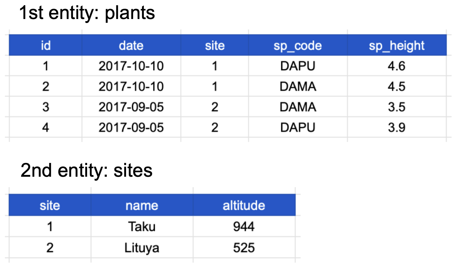
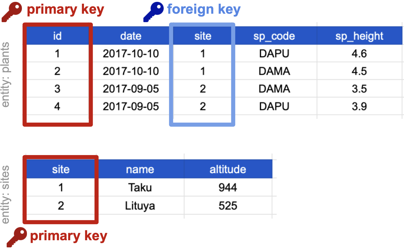
On our previously normalized data for plants and sites, let’s choose primary keys for these tables and then identify any foreign keys.
For the plants table:
- Notice that the columns
date, site and sp_code have repeated values across rows, thus cannot be primary keys.
- The columns
sp_height and id both have different values in each row, so both are candidates for primary keys.
- However, the decimal values of
sp_height don’t make it as useful to use it to reference observations
- and logically: if we take more observations, we may end up with multiple plants with the same height!
- So we chose
id as the primary key for this table.
For the sites table, all three columns could technically be keys as each column is unique. We chose site as the primary key because it is the most succinct and it also allows us to link the sites table with the plants table. (and again, logically, as we add more sites, can we guarantee that no two sites would have the same altitude?)
The site column is the primary key of the sites table because it uniquely identifies each row of the table as a unique observation of a site. In the plants table, however, the site column is a foreign key that references the primary key from the sites table.
This linkage tells us that the first height measurement for the DAPU observation occurred at the site with the name Taku.
Compound keys
It can also be the case that a single variable is not unique in itself so cannot be used as a key, but by combining it with a second variable, the combined values uniquely identify the rows.
This is called a Compound Key: a key that is made up of more than one variable.
For example, the site and sp_code columns in the plants table cannot be keys on their own, since each has repeated values. However, when we look at their combined values (1-DAPU, 1-DAMA, 2-DAMA, 2-DAPU) we see each row has a unique value. So site and sp_code together form a compound key: one unique observation of a specific plant at a specific site.
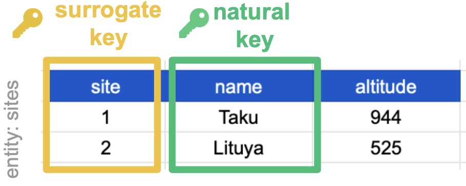
Primary and foreign keys are the workhorses of relational data, but there are also other types of keys, like natural keys or surrogate keys that can help you understand and communicate the connections within and between your data tables.
You can read more about this in this article.
Joins
Frequently, analysis of data will require merging these separately managed tables back together. There are multiple ways to join the observations in two tables, based on how the rows of one table are merged with the rows of the other. Regardless of the join we will perform, we need to start by identifying the primary key in each table and how these appear as foreign keys in other tables.
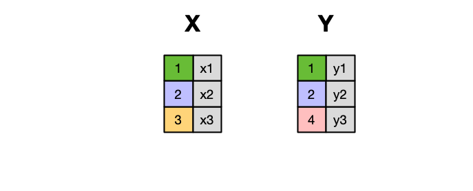
When conceptualizing merges, one can think of two tables, one on the left and one on the right.
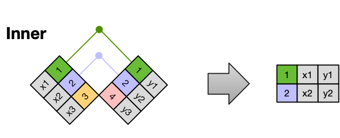
An INNER JOIN is when you merge the subset of rows that have matches in both the left table and the right table.
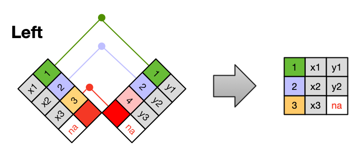
A LEFT JOIN takes all of the rows from the left table, and merges on the data from matching rows in the right table. Keys that don’t match from the left table are still provided with a missing value (na) from the right table.
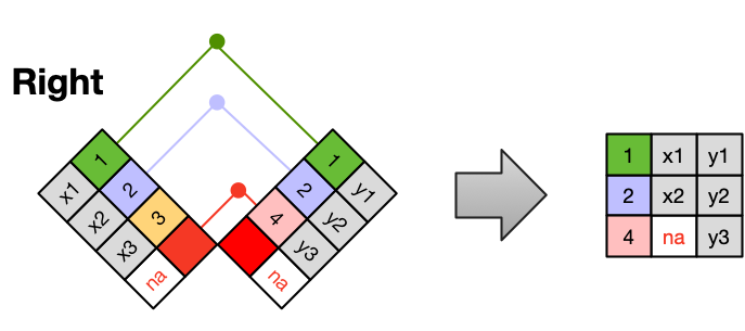
A RIGHT JOIN is the same as a left join, except that all of the rows from the right table are included with matching data from the left, or a missing value. Notice that left and right joins can ultimately be the same depending on the positions of the tables
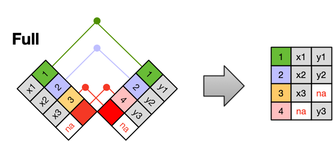
Finally, a FULL OUTER JOIN includes all data from all rows in both tables, and includes missing values wherever necessary.
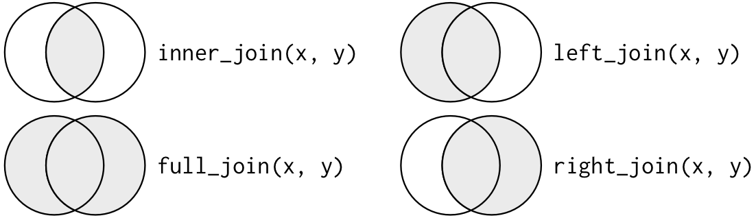
Sometimes people represent joins as Venn diagrams, showing which parts of the left and right tables are included in the results for each join. This representation is useful, however, they miss part of the story related to where the missing value comes from in each result.
We suggest reading the Relational Data chapter in the “R for Data Science” book for more examples and best practices about joins.
Entity-Relationship models
An Entity-Relationship model (E-R model), also known as an E-R diagram, is a way to draw a compact diagram that reflects the structure and relationships of the tables in a relational database. These can be particularly useful for big databases that have many tables and complex relationships between them.
These slides walk us through a simple example using our plants-sites dataset.
Full Screen
Best Practices Summary
The tidy data principles are:
- Every column is a variable.
- Every row is an observation.
- Every cell is a single value.
In normalized data we organize data so that:
- Each type of entity measured has its own table
- Observations (rows) are all unique
- Each column represents either an identifying variable or a measured variable
- Each table follows the tidy data principles
Creating relational data models by assigning primary and foreign keys to each table allows us to maintain relationships between separate normalized tables. Choose the primary key for each table based on your understanding of the data, and take efficiency into account. Once you choose a column as the primary key, make sure that all the values in that column are there!
For a big relational database, an Entity-Relationship model can be an effective way to explain how different tables and their keys are related to each other.
If we need to merge tables we can do it using different types of joins.
Tidy data is one very important step to data management best practices. However there is more to consider! Here are several tips from a great paper called ‘Some Simple Guidelines for Effective Data Management’.
- Design tables to add rows, not columns
- Use a scripted program (like R!)
- Non-proprietary file formats are preferred (eg: csv, txt)
- Keep a raw version of data
- Use descriptive files and variable names (without spaces!)
- Include a header line in your tabular data files
- Use plain ASCII text
Activity
- Get together in pairs or small groups
- Obtain materials from instructors including activity handout and blank paper(s).
- Follow instructions in activity handout.