### think of this code as someone saying "fave_num gets 42".
fave_num <- 42

### and then square it
fave_squared <- fave_num^2
fave_squared
[1] 1764This lesson is a combination of excellent lessons by others. Huge thanks to Julie Lowndes for writing most of this content and letting us build on her material, which in turn was built on Jenny Bryan’s materials. We highly recommend reading through the original lessons and using them as reference (see in the resources section below).
There is a vibrant community out there that is collectively developing increasingly easy to use and powerful open source programming tools. The changing landscape of programming is making learning how to code easier than it ever has been. Incorporating programming into analysis workflows not only makes science more efficient, but also more computationally reproducible. In this course, we will use the programming language R, and the accompanying integrated development environment (IDE) RStudio. R is a great language to learn for data-oriented programming because it is widely adopted, user-friendly, and (most importantly) open source.
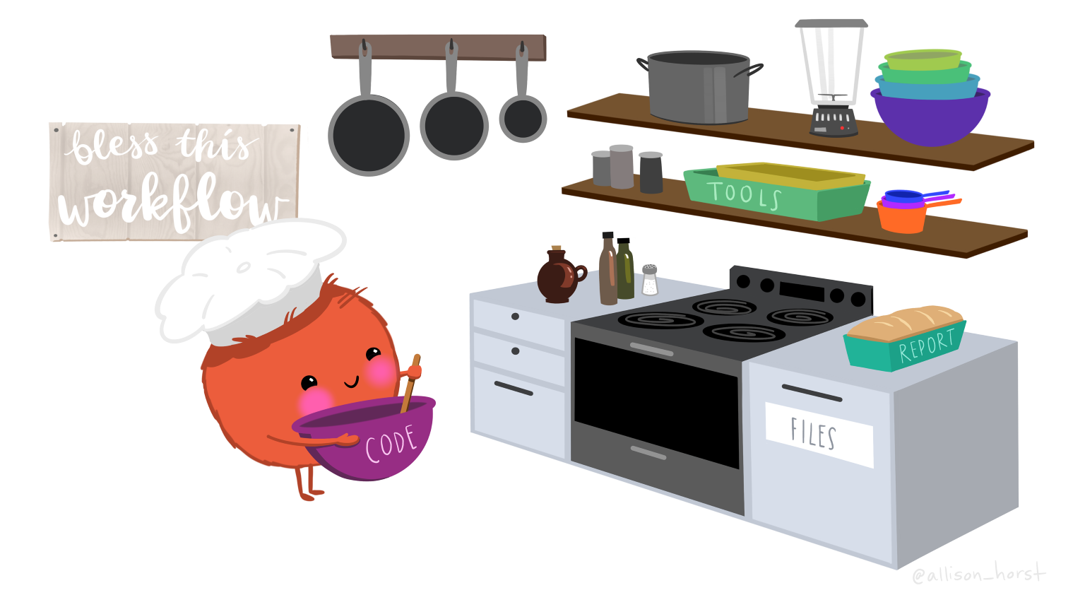
So what is the difference between R and RStudio? Here is an analogy to start us off. Imagine you are a chef, and you have to prepare a meal. You’ll need a place to work (a kitchen), you’ll need some tools (pots, pans, a knife, etc), and you’ll need some ingredients. In this analogy, R is a good chef’s knife - one of the most important tools that you’ll use to accomplish your task.
And if R is your chef’s knife, RStudio is your kitchen. RStudio provides a place to do your work! RStudio makes your life as a researcher easier by bringing together other tools you need to do your work efficiently - like a file browser, data viewer, help pages, terminal, community, support, the list goes on. So it’s not just the infrastructure (the user interface or IDE), although it is a great way to learn and interact with your variables, files, and interact directly with git. It’s also data science philosophy, R packages, community, and more.
(and in this analogy, your ingredients are data!)
Just as you can prepare food without a kitchen, we could learn R without RStudio, but that’s not what we’re going to do. RStudio makes it much easier to work with R, just as a well stocked kitchen makes cooking more fun. We are going to take advantage of the great RStudio support, and learn R and RStudio together.
Something else to start us off is to mention that you are learning a new language here. It’s an ongoing process, it takes time, you’ll make mistakes, it can be frustrating, but it will be overwhelmingly awesome in the long run. We all speak at least one language; it’s a similar process, really. And no matter how fluent you are, you’ll always be learning, you’ll be trying things in new contexts, learning words that mean the same as others, etc, just like everybody else. And just like any form of communication, there will be miscommunication that can be frustrating, but hands down we are all better off because of it.
While language is a familiar concept, programming languages are in a different context from spoken languages and you will understand this context with time. For example: you have a concept that there is a first meal of the day, and there is a name for that: in English it’s “breakfast.” So if you’re learning Spanish, you could expect there is a word for this concept of a first meal. (And you’d be right: “desayuno”). We will get you to expect that programming languages also have words (called functions) for concepts as well. You’ll soon expect that there is a way to order values numerically. Or alphabetically. Or search for patterns in text. Or calculate the median. Or reorganize columns to rows. Or subset exactly what you want. We will get you to increase your expectations and learn to ask and find what you’re looking for.
Let’s take a tour of the RStudio interface.
Let’s say the value of 12 that we got from running 3 * 4 is a really important value we need to keep. To keep information in R, we need to create an object. The way information is stored in R is through objects.
We can assign a value of a mathematical operation (and more!) to an object in R using the assignment operator, <- (greater than sign and minus sign). All objects in R are created using the assignment operator, following this form: object_name <- value.
When you begin typing an object name RStudio will automatically show suggested completions for you that you can select by hitting tab, then press return.
When you’re in the Console use the up and down arrow keys to call your command history, with the most recent commands being shown first.
Before we run more calculations, let’s talk about naming objects. For the object fave_num we used an underscore to separate the object name. This naming convention is called snake case. There are other naming conventions including, but not limited to:
we_used_snake_casesomeUseCamelCaseSomeUseUpperCamelCaseAlsoCalledPascalCaseChoosing a naming convention is a personal preference, but once you choose one, or your collaborative team chooses one - be consistent! A consistent naming convention will increase the readability of your code for others and your future self.
Object names cannot start with a numeric digit and cannot contain certain characters such as commas, spaces, or hyphens.
So far we’ve been running code in the Console, let’s try running code in an R Script. An R Script is a simple text file. RStudio uses an R Script by copying R commands from text in the file and pastes them into the Console as if you were manually entering commands yourself.
We’ve been using primarily integer or numeric data types so far. Let’s create an object that has a string value or a character data type, i.e., text instead of numbers.
science_rocks <- "yes it does!""yes it does!" is a string, and R knows it’s text and not a number because it is surrounded by quotes " ".
This lead us to an important concept in programming: There are different “classes” or types of objects in R (or any other programming language). The operations you can do with an object will depend on what type of object it is because each object has their own specialized format, designed for a specific purpose. While 7 * 5 seems like a reasonable calculation, "banana" * "apple" doesn’t make much sense. But there are many cool things we can do with strings that we can’t do with numbers.
So far we’ve learned some of the basic syntax and concepts of R programming, and how to navigate RStudio, but we haven’t done any complicated or interesting programming processes yet. This is where functions come in! In R, an object is a noun while a function is a verb - functions do all our data science work for us.
Let’s create a vector to store the noon temperature (in Celsius) in Santa Barbara for three consecutive summer days:
temp_c <- c(25, 29, 31)Now that we understand why the object’s value hasn’t changed - how do we update the value of mean_height_m? How is an R Script useful for this?
This lead us to another important programming concept, specifically for R Scripts: An R Script runs top to bottom.
This order of operations is important because if you are running code line by line, the values in object may be unexpected. When you are done writing your code in an R Script, it’s good practice to clear your Global Environment and use the Run button and select “Run all” to test that your R Script successfully runs top to bottom.
read.csv() function to read a file into RSo far we have learned how to assign values to objects in R, and what a function is, but we haven’t quite put it all together yet with real data yet. To do this, we will introduce the function read.csv(), which will be in the first lines of many of your future scripts. It does exactly what it says, it reads in a csv file to R.
Since this is our first time using this function, first access the help page for read.csv(). This has a lot of information in it, as this function has a lot of arguments, and the first one is especially important - we have to tell it what file to look for. Let’s get a file!
BGchem2008data.csv by clicking the “download” button next to the file (cloud with down arrow).
data in the same place as your script.data directory in your R project, click “Choose File,” and locate the BGchem2008data.csv file. Press “OK” to upload the file.data folder in the Files pane.Now we have to tell read.csv() how to find the file. We do this using the file argument which you can see in the usage section in the help page. In R, you can either use absolute paths (which will start with your home directory ~/) or paths relative to your current working directory. RStudio has some great auto-complete capabilities when using relative paths, so we will go that route.
Assuming you have moved your file to a folder within training_{USERNAME} called data, and your working directory is your project directory (training_{USERNAME}) your read.csv() call will look like this:
# reading in data using relative paths
bg_chem_dat <- read.csv(file = "data/BGchem2008data.csv")
You should now have an object of the class data.frame in your environment called bg_chem_dat. Check your environment pane to ensure this is true. Or you can check the class using the function class() in the console.
Notice that in the Help page there are many arguments that we didn’t use in the call above. Some of the arguments in function calls are optional, and some are required.
Optional arguments will be shown in the usage section with a name = value pair, with the default value shown. If you do not specify a name = value pair for that argument in your function call, the function will assume the default value (example: header = TRUE for read.csv()).
Required arguments will only show the name of the argument, without a value. Note that the only required argument for read.csv() is file.
You can always specify arguments in name = value form. But if you do not, R attempts to resolve by position. So above, it is assumed that we want file = "data/BGchem2008data.csv", since file is the first argument.
If we explicitly called the file argument our code would like this:
bg_chem_dat <- read.csv(file = "data/BGchem2008data.csv")If we wanted to add another argument, say stringsAsFactors, we need to specify it explicitly using the name = value pair, since the second argument is header.
Many R users (including myself) will set the stringsAsFactors argument using the following call:
# relative file path
bg_chem_dat <- read.csv("data/BGchem2008data.csv", stringsAsFactors = FALSE)For functions that are used often, you’ll see many programmers will write code that does not explicitly call the first or second argument of a function. For unfamiliar or uncommon functions, it’s a good idea to explicitly call the names of each argument - so your collaborators (including future-you!) can quickly understand the code.
Remember, a data.frame is a data structure in R that can represent tables and spreadsheets. It is a collection of rows and columns of data, where each column has a name and represents a variable, and each row represents an observation containing a measurement of that variable. When we ran read.csv(), we read the file data into a data.frame and then saved the result in the object bg_chem_dat. Explore the dataset:
bg_chem_dat in the environment panebg_chem_dat in the environment panehead(bg_chem_dat) in the ConsoleView(bg_chem_dat) in the ConsoleLet’s examine specific columns and run some basic calculations, using R functions. Try these, try out other functions and calculations. Can you calculate the standard deviation or sum? Don’t worry, if you try something and don’t get it right, nothing bad will happen - at worst, you get an error message and try again.
head(bg_chem_dat$Date)

mean_temp <- mean(bg_chem_dat$CTD_Temperature)While the base R package provides read.csv as a common way to load tabular data from text files, there are many other ways that can be convenient and will also produce a data.frame as output. Here are a few:
readr::read_csv() function from the Tidyverse to load the data file. The readr package has a bunch of convenient helpers and handles CSV files in typically expected ways, like properly typing dates and time columns. bg_chem_dat <- readr::read_csv("data/BGchem2008data.csv")readxl::read_excel() function.googlesheets4::read_sheet() function.We can ask questions about an object using logical operators and expressions. Let’s ask some “questions” about the tree_h_m object we made.
== means ‘is equal to’!= means ‘is not equal to’< means ‘is less than’> means ‘is greater than’<= means ‘is less than or equal to’>= means ‘is greater than or equal to’R will apply the logical test to each element of a vector and tell you the result as TRUE or FALSE.
# examples using logical operators and expressions
tree_h_m == 8.9
[1] FALSE FALSE FALSE FALSE FALSEtree_h_m >= 14[1] TRUE FALSE TRUE TRUE TRUEtree_h_m != 11.3[1] TRUE TRUE TRUE TRUE TRUE
There is an implicit contract with the computer/scripting language: Computer will do tedious computation for you. In return, you the user will be completely precise in your instructions. Typos matter. Case matters. Pay attention to how you type.
Remember that this is a language, not dissimilar to English! There are times you aren’t understood – it’s going to happen. There are different ways this can happen. Sometimes you’ll get an error. This is like someone saying ‘What?’ or ‘Pardon’? Error messages can also be more useful, like when they say ‘I didn’t understand this specific part of what you said, I was expecting something else’. That is a great type of error message. Other times they are inscrutable. Those are not great.
Error messages are a learning opportunity. Use Google or ChatGPT (copy-and-paste!) to figure out what they mean. Note that knowing how to Google is a skill and takes practice - use our Masters of Environmental Data Science (MEDS) program workshop Teach Me How to Google as a guide.
And also know that there are errors that can creep in more subtly, without an error message right away, when you are giving information that is understood, but not in the way you meant. Like if I’m telling a story about tables and you’re picturing where you eat breakfast and I’m talking about data. This can leave me thinking I’ve gotten something across that the listener (or R) interpreted very differently. And as I continue telling my story you get more and more confused… So write clean code and check your work as you go to minimize these circumstances!

R packages are the building blocks of computational reproducibility in R. Each package contains a set of related functions that enable you to more easily do a task or set of tasks in R. There are thousands of community-maintained packages out there for just about every imaginable use of R - including many that you have probably never thought of!
To install a package, we use the syntax install.packages("packge_name"). A package only needs to be installed once, so this code can be run directly in the console if needed. Generally, you don’t want to save your install package calls in a script, because when you run the script it will re-install the package, which you only need to do once, or if you need to update the package.
| Learning R Resources |
|
| Community Resources |
|
| Cheatsheets |
Take a look at the objects in your Environment (Workspace) in the upper right pane. The Workspace is where user-defined objects accumulate. There are a few useful commands for getting information about your Environment, which make it easier for you to reference your objects when your Environment gets filled with many, many objects.
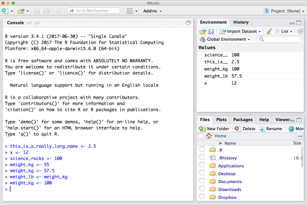
You can get a listing of these objects with a couple of different R functions:
objects() [1] "fave_num" "fave_squared" "m_to_ft" "mean_height_m"
[5] "mean_temp_c" "mtcars" "science_rocks" "temp_c"
[9] "tree_h_ft" "tree_h_m" "x" "y"
[13] "z" ls() [1] "fave_num" "fave_squared" "m_to_ft" "mean_height_m"
[5] "mean_temp_c" "mtcars" "science_rocks" "temp_c"
[9] "tree_h_ft" "tree_h_m" "x" "y"
[13] "z" If you want to remove the object named tree_h_m, you can do this:
rm(tree_h_m)To remove everything (or click the Broom icon in the Environment pane):
rm(list = ls())It’s good practice to clear your environment. Over time your Global Environmental will fill up with many objects, and this can result in unexpected errors or objects being overridden with unexpected values. Also it’s difficult to read / reference your environment when it’s cluttered!
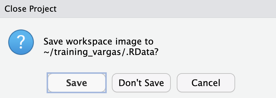
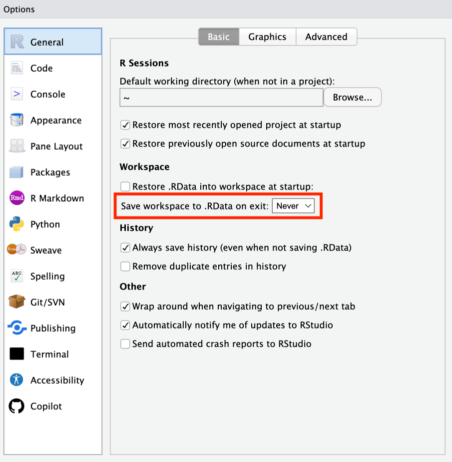
DON’T SAVE
When ever you close or switch projects you will be promped with the question: Do you want to save your workspace image to /“current-project”/ .RData?
RStudio by default wants to save the state of your environment (the objects you have in your environment pane) into the RData file so that when you open the project again you have the same environment. However, as we discussed above, it is good practice to constantly clear and clean your environment. It is generally NOT a good practice to rely on the state of your environment for your script to run and work. If you are coding reproducibly, your code should be able to reproduce the state of your environment (all the necessary objects) every time you run it. It is much better to rely on your code recreating the environment than saving the workspace status.
To make sure you’re always working reproducibly, change the Global Options configuration for the default to be NEVER SAVE MY WORKSPACE. Go to Tools > Global Options. Under the General menu, select Never next to “Save workspace to .RData on exit” (and uncheck “Restore .RData into workspace at startup”). This way you won’t get asked every time you close a project, instead RStudio knows not to save.